Examples for installation checking

The examples below show how to run VIA on generic connected and disconnected data using wrapper functions and serve as a check for your installation. For more detailed guidelines on running VIA and plotting the results, please use the Notebooks. We also highlight a few difference in calling VIA when using Windows versus Linux. The data for the Jupyter Notebooks and Examples are available in the Datasets folder (smaller files) with larger datasets here

A test script is available for some of the different datasets, please change the foldername accordingly to the folder containing relevant data files

1.a Toy Data (multifurcation) Multifurcation Jupyter NB
1.b Toy Data (disconnected) Disconnected Jupyter NB
2.a General input data formatting and wrapper function
2.b General disconnected trajectories wrapper function
3.a Human Embryoid Bodies (wrapper function for testing VIA)
3.b Human Embryoid Bodies (Configuring VIA) EB Jupyter NB

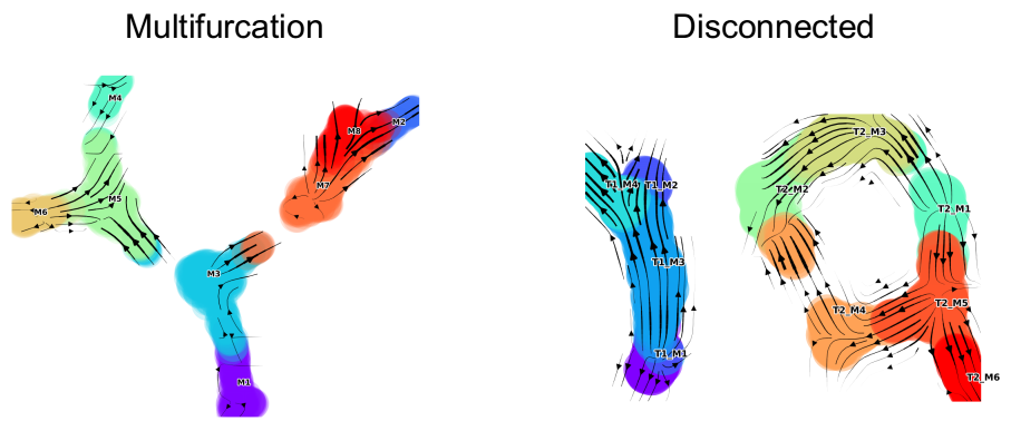
1.a/b Toy data (Multifurcation and Disconnected)

Two examples toy datasets with annotations generated using DynToy are provided. For the step-by-step code within these wrappers, please see the corresponding Jupyter NBs.

1.a/b Run on Linux

All examples are shown according to Linux OS, small modifications are required to run on a Windows OS (see below):

import pyVIA.core as via
# ensure the data and label files are in csv format when you download/save them
# multifurcation
# the root is automatically set to  root_user = 'M1'
via.main_Toy(ncomps=10, knn=30,dataset='Toy3', random_seed=2,foldername = ".../Trajectory/Datasets/") #multifurcation
# disconnected trajectory
# In the wrapper for Toy, the root is automatically set as a list root_user = ['T1_M1', 'T2_M1'] # e.g. T2_M3 is a cell belonging to the 3rd Milestone (M3) of the   second Trajectory (T2)
via.main_Toy(ncomps=10, knn=30,dataset='Toy4',random_seed=2,foldername =".../Trajectory/Datasets/") #2 disconnected trajectories

1.a/b Run on Windows

Windows may require minor modifications in calling the code due to the way multiprocessing works in Windows compared to Linux:

#when running from an IDE you need to call the function in the following way to ensure the parallel processing works:
import os
import pyVIA.core as via
f= os.path.join(r'C:\Users\...\Documents'+'\\')
def main():
    via.main_Toy(ncomps=10, knn=30,dataset='Toy3', random_seed=2,foldername= f)
if __name__ =='__main__':
    main()

#when running directly from terminal:
import os
import pyVIA.core as via
f= os.path.join(r'C:\Users\...\Documents'+'\\')
via.main_Toy(ncomps=10, knn=30,dataset='Toy3', random_seed=2,foldername= f)

**Multifurcating toy dataset 1.a ** *(click to open interactive graph)*

Disconnected toy dataset 1.b (click to open interactive graph)

2.a General input format and wrapper function (uses example of pre-B cell differentiation)

These wrapper functions are a good start but we highly recommend you look at the tutorials as you will be afforded a much higher degree of control without much added complexity. The below wrappers operate in the 2-iteration format (a coarse followed by a fine-grained), but this is not always needed and you will have more intuitive for the behaviour of your data by following the steps in the Tutorials. Nonetheless, the following wrappers are a great way to start to familiarize yourself with the various outputs from VIA.

Datasets and labels used in this example are provided in Datasets

# Read the two files:
# 1) The first file contains 200PCs of the Bcell filtered and normalized data for the first 5000 HVG.
# 2) The second file contains raw count data for marker genes

data = pd.read_csv('./Bcell_200PCs.csv')
data_genes = pd.read_csv('./Bcell_markergenes.csv')
data_genes = data_genes.drop(['cell'], axis=1)
true_label = data['time_hour']
data = data.drop(['cell', 'time_hour'], axis=1)
adata = sc.AnnData(data_genes)
adata.obsm['X_pca'] = data.values

# use UMAP or PHate to obtain embedding that is used for single-cell level visualization
embedding = umap.UMAP(random_state=42, n_neighbors=15, init='random').fit_transform(data.values[:, 0:5])

# list marker genes or genes of interest if known in advance. otherwise marker_genes = []
marker_genes = ['Igll1', 'Myc', 'Slc7a5', 'Ldha', 'Foxo1', 'Lig4', 'Sp7']  # irf4 down-up
# call VIA. We identify an early (suitable) start cell root = [42]. Can also set an arbitrary value
via.via_wrapper(adata, true_label, embedding, knn=10, ncomps=20, jac_std_global=0.15, root=[42], dataset='',
            random_seed=1,v0_toobig=0.3, v1_toobig=0.1, marker_genes=marker_genes)

2.b VIA wrapper for generic disconnected trajectory

A slightly different wrapper is called for the disconnected scenario. Refer to the Jupytern NB for a step-by-step tutorial.:

import scanpy as sc
import pandas as pd

#foldername corresponds to the location where you have saved the Toy Disconnected data (shown in example 2)
#Read in the data and labels
df_counts = pd.read_csv(foldername + "toy_disconnected_M9_n1000d1000.csv", 'rt', delimiter=",")
df_ids = pd.read_csv(foldername + "toy_disconnected_M9_n1000d1000_ids.csv", 'rt', delimiter=",")

# Make AnnData object for wrapper function to read-in data and do PCA
df_ids['cell_id_num'] = [int(s[1::]) for s in df_ids['cell_id']]
df_counts = df_counts.drop('Unnamed: 0', 1)
df_ids = df_ids.sort_values(by=['cell_id_num'])
df_ids = df_ids.reset_index(drop=True)
true_label = df_ids['group_id']
adata_counts = sc.AnnData(df_counts, obs=df_ids)
sc.tl.pca(adata_counts, svd_solver='arpack', n_comps=10)

#Since there are 2 disconnected trajectories, we provide 2 arbitrary roots (start cells).If there are more disconnected paths, then VIA arbitrarily selects roots. #The root can also just be arbitrarily set as [1] and VIA can detect how many additional roots it must add
# The root can also be provided as a cell type level label corresponding to the groups present in "true_label", in this case the dataset must be set to 'group'
via.via_wrapper_disconnected(adata_counts, true_label, embedding=adata_counts.obsm['X_pca'][:, 0:2], root=[1,1], preserve_disconnected=True, knn=30, ncomps=10,cluster_graph_pruning_std = 1)

#in the case of connected data (i.e. only 1 graph component. e.g. Toy Data Multifurcating) then the wrapper function from example 3.a can be used:
via.via_wrapper(adata_counts, true_label, embedding=  adata_counts.obsm['X_pca'][:,0:2], root=[1], knn=30, ncomps=10,cluster_graph_pruning_std = 1)