StaVia for scATAC-seq Hematopoiesis
We show an example of automated cell fate prediction and pathway determination, and visualization for TI, on a scATAC-seq dataset
import pandas as pd
import matplotlib.pyplot as plt
import pyVIA.core as via
import warnings
warnings.filterwarnings('ignore')
#data available on StaVia's github page as a csv file, containing the TFs, cell annotations and Principle Components used in the original paper by Buenrostro et al.,
df = pd.read_csv('/home/user/Trajectory/Datasets/scATAC_Hemato/scATAC_hemato_Buenrostro.csv', sep=',')
print('number cells', df.shape[0])
cell_types = ['GMP', 'HSC', 'MEP', 'CLP', 'CMP', 'LMuPP', 'MPP', 'pDC', 'mono', 'UNK']
cell_dict = {'UNK': 'gray', 'pDC': 'purple', 'mono': 'gold', 'GMP': 'orange', 'MEP': 'red', 'CLP': 'aqua',
                 'HSC': 'black', 'CMP': 'moccasin', 'MPP': 'darkgreen', 'LMuPP': 'limegreen'}
cell_annot = df['cellname'].values


true_label = []
count = 0
found_annot = False
#reformatting the celltype labels
for annot in cell_annot:
    for cell_type_i in cell_types:
        if cell_type_i in annot:
            true_label.append(cell_type_i)
            found_annot = True

    if found_annot == False:
        true_label.append('unknown')
    found_annot = False

PCcol = ['PC1', 'PC2', 'PC3', 'PC4', 'PC5'] #columns in the dataframe containing the Principle Components from the TFs. details of the preprocessing method are described in Buenrostro's paper
number cells 2034
knn = 20
random_seed = 4
X_in = df[PCcol].values  #using the PCs provided in the Buenrostro et al., paper

start_ncomp = 0
root = [1200] #the 1200th cell in the input is an HSC cell

v0 = via.VIA(X_in, true_label, edgepruning_clustering_resolution=0.5, edgepruning_clustering_resolution_local=1, knn=knn,
         too_big_factor=0.3, root_user=root, dataset='', random_seed=random_seed, memory = 2,
          preserve_disconnected=False)
v0.run_VIA()
2024-02-15 17:29:20.222939	Running VIA over input data of 2034 (samples) x 5 (features)
2024-02-15 17:29:20.223006	Knngraph has 20 neighbors
2024-02-15 17:29:22.628608	Finished global pruning of 20-knn graph used for clustering at level of 0.5. Kept 63.6 % of edges.
2024-02-15 17:29:22.643187	Number of connected components used for clustergraph  is 1
2024-02-15 17:29:22.751012	Commencing community detection
2024-02-15 17:29:22.785685	Finished running Leiden algorithm. Found 31 clusters.
2024-02-15 17:29:22.787772	Merging 4 very small clusters (<10)
2024-02-15 17:29:22.789018	Finished detecting communities. Found 27 communities
2024-02-15 17:29:22.789580	Making cluster graph. Global cluster graph pruning level: 0.15
2024-02-15 17:29:22.797542	Graph has 1 connected components before pruning
2024-02-15 17:29:22.800130	Graph has 5 connected components after pruning
2024-02-15 17:29:22.805491	Graph has 1 connected components after reconnecting
2024-02-15 17:29:22.806314	0.0% links trimmed from local pruning relative to start
2024-02-15 17:29:22.806351	52.4% links trimmed from global pruning relative to start
2024-02-15 17:29:22.810292	component number 0 out of  [0]
2024-02-15 17:29:22.816664	The root index, 1200 provided by the user belongs to cluster number 21 and corresponds to cell type HSC
2024-02-15 17:29:22.820309	Computing lazy-teleporting expected hitting times
2024-02-15 17:29:23.687191	 ended all multiprocesses, will retrieve and reshape
try rw2 hitting times setup
start computing walks with rw2 method
g.indptr.size, 28
memory for rw2 hittings times  2. Using rw2 based pt
do scaling of pt
2024-02-15 17:29:30.199701	Identifying terminal clusters corresponding to unique lineages...
2024-02-15 17:29:30.199736	Closeness:[6, 15, 17, 20, 22, 23, 24, 25, 26]
2024-02-15 17:29:30.199751	Betweenness:[0, 1, 5, 6, 11, 15, 16, 17, 20, 21, 22, 23, 24, 25, 26]
2024-02-15 17:29:30.199766	Out Degree:[5, 6, 7, 11, 13, 15, 17, 18, 20, 24, 25, 26]
2024-02-15 17:29:30.200347	Terminal clusters corresponding to unique lineages in this component are [5, 6, 11, 15, 17, 20, 22, 23, 24, 25, 26]
TESTING rw2_lineage probability at memory 2
testing rw2 lineage probability at memory 2
g.indptr.size, 28
2024-02-15 17:29:36.281404	 Cluster or terminal cell fate 5 is reached 657.0 times
2024-02-15 17:29:36.377637	 Cluster or terminal cell fate 6 is reached 598.0 times
2024-02-15 17:29:36.468722	 Cluster or terminal cell fate 11 is reached 224.0 times
2024-02-15 17:29:36.576330	 Cluster or terminal cell fate 15 is reached 146.0 times
2024-02-15 17:29:36.674248	 Cluster or terminal cell fate 17 is reached 90.0 times
2024-02-15 17:29:36.746055	 Cluster or terminal cell fate 20 is reached 596.0 times
2024-02-15 17:29:36.842464	 Cluster or terminal cell fate 22 is reached 142.0 times
2024-02-15 17:29:36.947835	 Cluster or terminal cell fate 23 is reached 134.0 times
2024-02-15 17:29:37.057720	 Cluster or terminal cell fate 24 is reached 119.0 times
2024-02-15 17:29:37.165999	 Cluster or terminal cell fate 25 is reached 121.0 times
2024-02-15 17:29:37.288452	 Cluster or terminal cell fate 26 is reached 119.0 times
2024-02-15 17:29:37.315628	There are (11) terminal clusters corresponding to unique lineages {5: 'CMP', 6: 'MEP', 11: 'GMP', 15: 'pDC', 17: 'mono', 20: 'MEP', 22: 'pDC', 23: 'pDC', 24: 'CLP', 25: 'CLP', 26: 'pDC'}
2024-02-15 17:29:37.315691	Begin projection of pseudotime and lineage likelihood
2024-02-15 17:29:37.578716	Cluster graph layout based on forward biasing
2024-02-15 17:29:37.582665	Starting make edgebundle viagraph...
2024-02-15 17:29:37.582696	Make via clustergraph edgebundle
2024-02-15 17:29:37.832212	Hammer dims: Nodes shape: (27, 2) Edges shape: (64, 3)
2024-02-15 17:29:37.834641	Graph has 1 connected components before pruning
2024-02-15 17:29:37.838025	Graph has 9 connected components after pruning
2024-02-15 17:29:37.850265	Graph has 1 connected components after reconnecting
2024-02-15 17:29:37.851195	23.3% links trimmed from local pruning relative to start
2024-02-15 17:29:37.851239	45.0% links trimmed from global pruning relative to start
2024-02-15 17:29:37.863579	Time elapsed 17.3 seconds
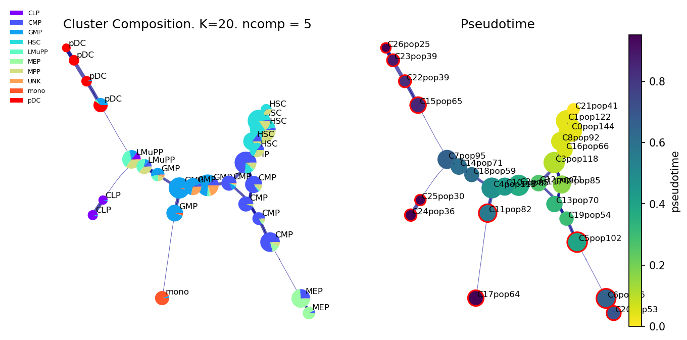
f,ax1, axs2 = via.plot_piechart_viagraph(v0)
f.set_size_inches(10,5)
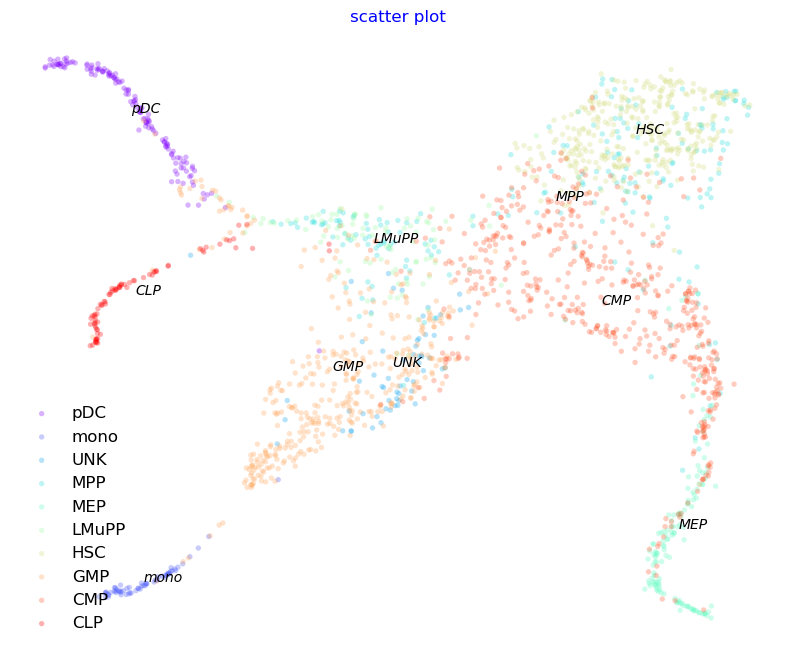
#Create 2D StaVia embedding using the underlying TI infused graph. The 2D embedding will be visually well aligned with the cluster-graph of the trajectory
embedding = via.via_atlas_emb(via_object=v0, min_dist=0.4) #StaVia's TI initialized embedding. Feel free to use a t-SNE, UMAP etc instead
f, ax = via.plot_scatter(embedding=embedding, labels=true_label, s=15)
f.set_size_inches(10,8)
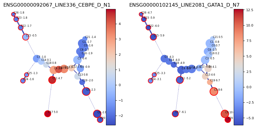
#plot the gene expression of selected genes along the clustergraph
df =df.drop(['cellname'], axis=1)
gene_dict = {  'ENSG00000092067_LINE336_CEBPE_D_N1': 'CEBPE Eosophil (GMP/Mono)','ENSG00000102145_LINE2081_GATA1_D_N7':'GATA1 (MEP)'}
genes_to_plot_list = ['ENSG00000092067_LINE336_CEBPE_D_N1','ENSG00000102145_LINE2081_GATA1_D_N7']
f, axs = via.plot_viagraph( via_object=v0,df_genes=df, gene_list=genes_to_plot_list)
f.set_size_inches(10,5)
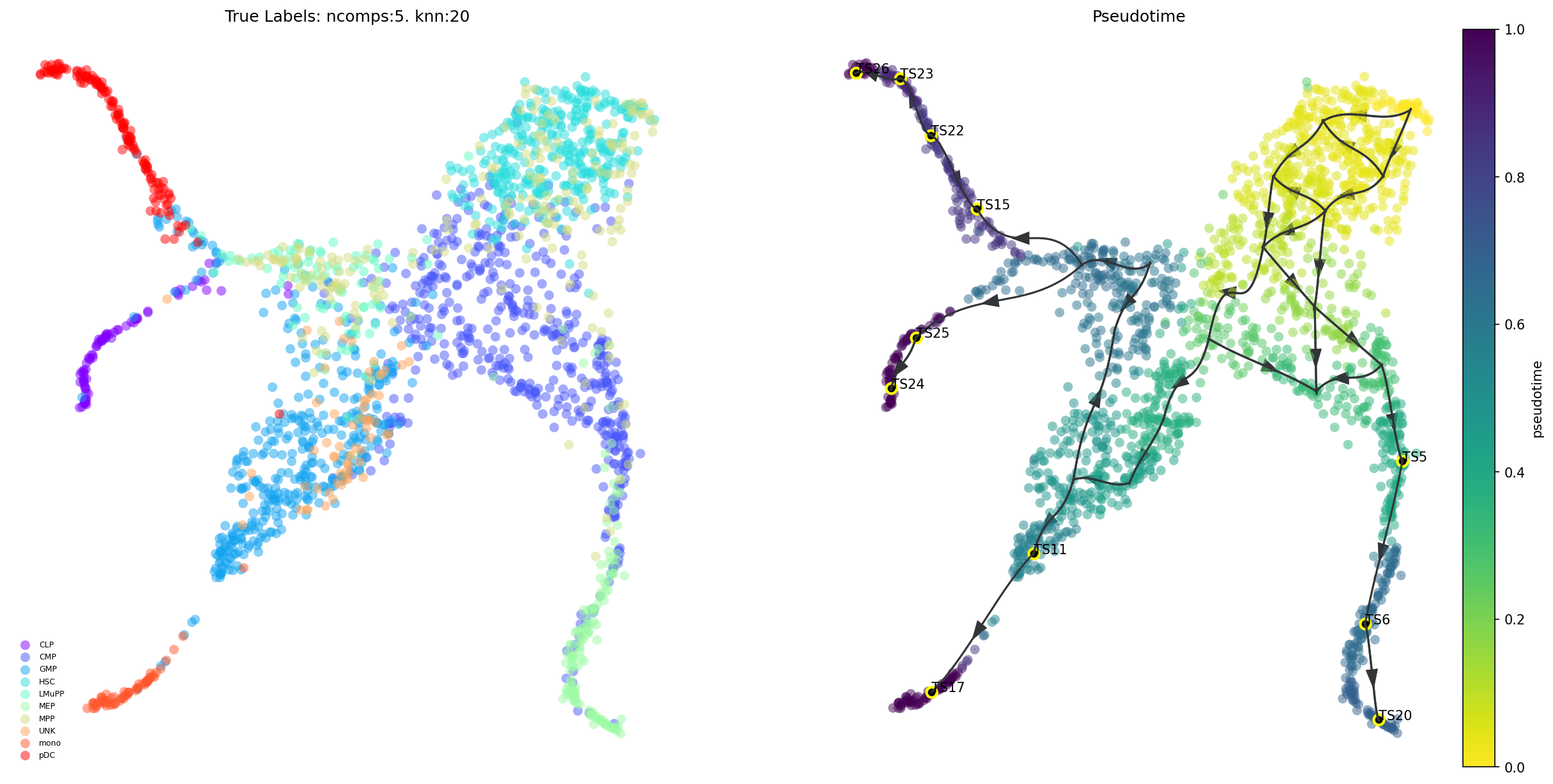
# draw overall pseudotime and main trajectories
via.plot_trajectory_curves(via_object = v0, embedding = embedding,
title_str='Pseudotime')
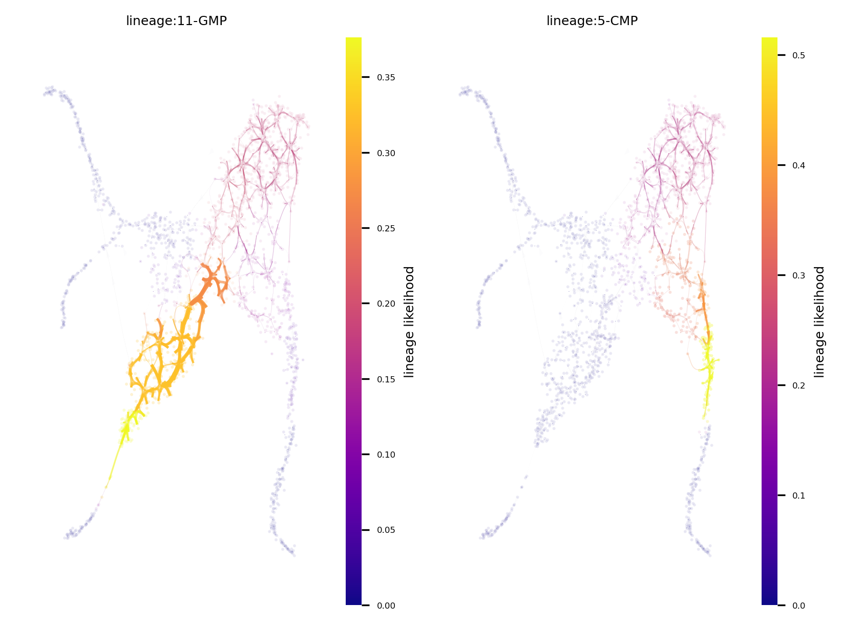
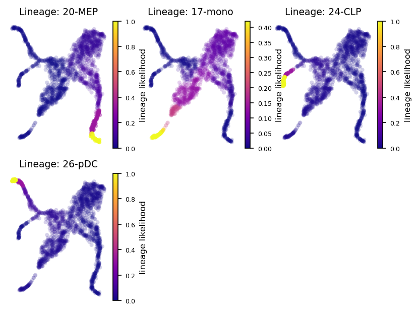
# draw trajectory and evolution probability for each lineage
100% (11 of 11) |########################| Elapsed Time: 0:00:00 Time:  0:00:00
100% (11 of 11) |########################| Elapsed Time: 0:00:00 Time:  0:00:00
100% (11 of 11) |########################| Elapsed Time: 0:00:00 Time:  0:00:00
100% (11 of 11) |########################| Elapsed Time: 0:00:00 Time:  0:00:00
100% (11 of 11) |########################| Elapsed Time: 0:00:00 Time:  0:00:00
100% (11 of 11) |########################| Elapsed Time: 0:00:01 Time:  0:00:01
100% (11 of 11) |########################| Elapsed Time: 0:00:00 Time:  0:00:00
100% (11 of 11) |########################| Elapsed Time: 0:00:00 Time:  0:00:00
100% (11 of 11) |########################| Elapsed Time: 0:00:00 Time:  0:00:00
100% (11 of 11) |########################| Elapsed Time: 0:00:00 Time:  0:00:00
100% (11 of 11) |########################| Elapsed Time: 0:00:00 Time:  0:00:00
100% (11 of 11) |########################| Elapsed Time: 0:00:00 Time:  0:00:00
100% (11 of 11) |########################| Elapsed Time: 0:00:00 Time:  0:00:00
100% (11 of 11) |########################| Elapsed Time: 0:00:00 Time:  0:00:00
100% (11 of 11) |########################| Elapsed Time: 0:00:00 Time:  0:00:00
100% (11 of 11) |########################| Elapsed Time: 0:00:00 Time:  0:00:00
100% (11 of 11) |########################| Elapsed Time: 0:00:00 Time:  0:00:00
100% (11 of 11) |########################| Elapsed Time: 0:00:00 Time:  0:00:00
100% (11 of 11) |########################| Elapsed Time: 0:00:00 Time:  0:00:00
100% (11 of 11) |########################| Elapsed Time: 0:00:00 Time:  0:00:00
100% (11 of 11) |########################| Elapsed Time: 0:00:00 Time:  0:00:00
100% (11 of 11) |########################| Elapsed Time: 0:00:00 Time:  0:00:00
100% (11 of 11) |########################| Elapsed Time: 0:00:00 Time:  0:00:00
100% (11 of 11) |########################| Elapsed Time: 0:00:00 Time:  0:00:00
100% (11 of 11) |########################| Elapsed Time: 0:00:00 Time:  0:00:00
100% (11 of 11) |########################| Elapsed Time: 0:00:00 Time:  0:00:00
100% (11 of 11) |########################| Elapsed Time: 0:00:00 Time:  0:00:00
100% (11 of 11) |########################| Elapsed Time: 0:00:00 Time:  0:00:00
100% (11 of 11) |########################| Elapsed Time: 0:00:00 Time:  0:00:00
100% (11 of 11) |########################| Elapsed Time: 0:00:00 Time:  0:00:00
100% (11 of 11) |########################| Elapsed Time: 0:00:00 Time:  0:00:00
100% (11 of 11) |########################| Elapsed Time: 0:00:00 Time:  0:00:00
100% (11 of 11) |########################| Elapsed Time: 0:00:00 Time:  0:00:00
100% (11 of 11) |########################| Elapsed Time: 0:00:00 Time:  0:00:00
100% (11 of 11) |########################| Elapsed Time: 0:00:00 Time:  0:00:00
100% (11 of 11) |########################| Elapsed Time: 0:00:00 Time:  0:00:00
100% (11 of 11) |########################| Elapsed Time: 0:00:00 Time:  0:00:00
100% (11 of 11) |########################| Elapsed Time: 0:00:00 Time:  0:00:00
100% (11 of 11) |########################| Elapsed Time: 0:00:00 Time:  0:00:00
100% (11 of 11) |########################| Elapsed Time: 0:00:00 Time:  0:00:00
2024-02-15 17:35:32.244532	Super cluster 5 is a super terminal with sub_terminal cluster 5
2024-02-15 17:35:32.244619	Super cluster 6 is a super terminal with sub_terminal cluster 6
2024-02-15 17:35:32.244658	Super cluster 11 is a super terminal with sub_terminal cluster 11
2024-02-15 17:35:32.244690	Super cluster 15 is a super terminal with sub_terminal cluster 15
2024-02-15 17:35:32.244719	Super cluster 17 is a super terminal with sub_terminal cluster 17
2024-02-15 17:35:32.244749	Super cluster 20 is a super terminal with sub_terminal cluster 20
2024-02-15 17:35:32.244776	Super cluster 22 is a super terminal with sub_terminal cluster 22
2024-02-15 17:35:32.244808	Super cluster 23 is a super terminal with sub_terminal cluster 23
2024-02-15 17:35:32.244834	Super cluster 24 is a super terminal with sub_terminal cluster 24
2024-02-15 17:35:32.244861	Super cluster 25 is a super terminal with sub_terminal cluster 25
2024-02-15 17:35:32.244886	Super cluster 26 is a super terminal with sub_terminal cluster 26
(<Figure size 3000x1500 with 3 Axes>,
 <Axes: title={'center': 'True Labels: ncomps:5. knn:20'}>,
 <Axes: title={'center': 'Pseudotime'}>)
via.plot_sc_lineage_probability(via_object=v0, embedding = embedding,marker_lineages=[20,17,24,26])
plt.show()
2024-02-15 17:35:48.454355	Marker_lineages: [20, 17, 24, 26]
2024-02-15 17:35:48.457705	The number of components in the original full graph is 1
2024-02-15 17:35:48.457755	For downstream visualization purposes we are also constructing a low knn-graph
2024-02-15 17:35:50.070895	Check sc pb 0.9999999999999999
f getting majority comp
2024-02-15 17:35:50.197961	Cluster path on clustergraph starting from Root Cluster 21 to Terminal Cluster 5: [21, 1, 8, 3, 9, 19, 5]
2024-02-15 17:35:50.198004	Cluster path on clustergraph starting from Root Cluster 21 to Terminal Cluster 6: [21, 1, 8, 3, 9, 19, 5, 6]
2024-02-15 17:35:50.198030	Cluster path on clustergraph starting from Root Cluster 21 to Terminal Cluster 11: [21, 1, 8, 3, 12, 2, 10, 4, 11]
2024-02-15 17:35:50.198055	Cluster path on clustergraph starting from Root Cluster 21 to Terminal Cluster 15: [21, 1, 8, 3, 12, 2, 10, 4, 18, 14, 7, 15]
2024-02-15 17:35:50.198081	Cluster path on clustergraph starting from Root Cluster 21 to Terminal Cluster 17: [21, 1, 8, 3, 12, 2, 10, 4, 11, 17]
2024-02-15 17:35:50.198106	Cluster path on clustergraph starting from Root Cluster 21 to Terminal Cluster 20: [21, 1, 8, 3, 9, 19, 5, 6, 20]
2024-02-15 17:35:50.198131	Cluster path on clustergraph starting from Root Cluster 21 to Terminal Cluster 22: [21, 1, 8, 3, 12, 2, 10, 4, 18, 14, 7, 15, 22]
2024-02-15 17:35:50.198157	Cluster path on clustergraph starting from Root Cluster 21 to Terminal Cluster 23: [21, 1, 8, 3, 12, 2, 10, 4, 18, 14, 7, 15, 22, 23]
2024-02-15 17:35:50.198182	Cluster path on clustergraph starting from Root Cluster 21 to Terminal Cluster 24: [21, 1, 8, 3, 12, 2, 10, 4, 18, 14, 7, 25, 24]
2024-02-15 17:35:50.198206	Cluster path on clustergraph starting from Root Cluster 21 to Terminal Cluster 25: [21, 1, 8, 3, 12, 2, 10, 4, 18, 14, 7, 25]
2024-02-15 17:35:50.198232	Cluster path on clustergraph starting from Root Cluster 21 to Terminal Cluster 26: [21, 1, 8, 3, 12, 2, 10, 4, 18, 14, 7, 15, 22, 23, 26]
2024-02-15 17:35:50.354424	Revised Cluster level path on sc-knnGraph from Root Cluster 21 to Terminal Cluster 20 along path: [21, 0, 13, 6, 20, 20, 20, 20, 20]
2024-02-15 17:35:50.397034	Revised Cluster level path on sc-knnGraph from Root Cluster 21 to Terminal Cluster 17 along path: [21, 0, 12, 10, 11, 17, 17, 17, 17, 17]
2024-02-15 17:35:50.438633	Revised Cluster level path on sc-knnGraph from Root Cluster 21 to Terminal Cluster 24 along path: [21, 21, 21, 1, 7, 25, 24, 24, 24]
2024-02-15 17:35:50.480060	Revised Cluster level path on sc-knnGraph from Root Cluster 21 to Terminal Cluster 26 along path: [21, 21, 21, 1, 7, 15, 23, 26, 26]
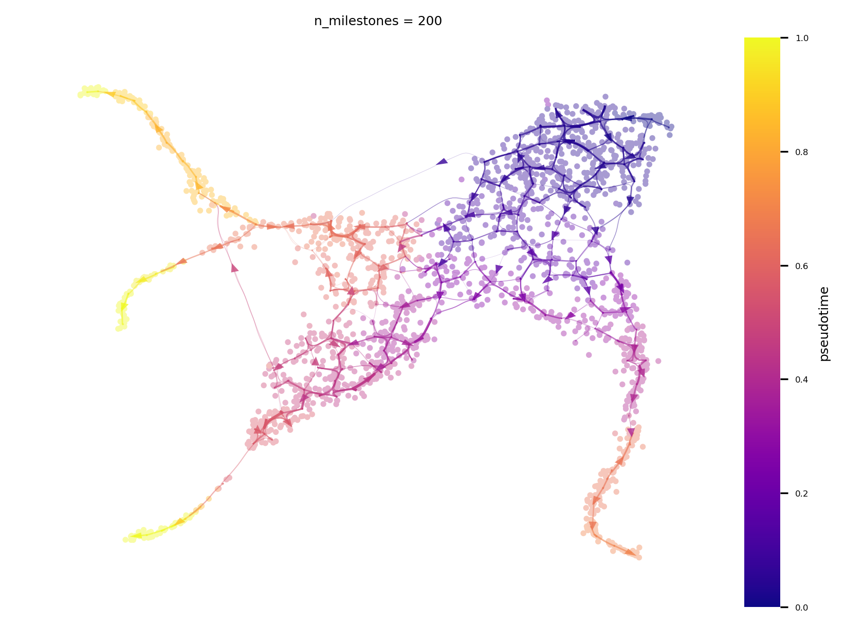
v0.embedding = embedding
f,ax = via.plot_atlas_view(via_object=v0,  n_milestones=200, add_sc_embedding=True, sc_labels_expression=v0.single_cell_pt_markov, headwidth_bundle=0.25, linewidth_bundle=2, size_milestones=1, sc_scatter_size=3)
2024-02-15 17:36:03.802544	Computing Edges
2024-02-15 17:36:03.802679	Start finding milestones
2024-02-15 17:36:07.042547	End milestones with 200
2024-02-15 17:36:07.047312	Recompute weights
2024-02-15 17:36:07.069225	pruning milestone graph based on recomputed weights
2024-02-15 17:36:07.070744	Graph has 1 connected components before pruning
2024-02-15 17:36:07.071944	Graph has 1 connected components after pruning
2024-02-15 17:36:07.072208	Graph has 1 connected components after reconnecting
2024-02-15 17:36:07.073549	regenerate igraph on pruned edges
2024-02-15 17:36:07.081077	Setting numeric label as time_series_labels or other sequential metadata for coloring edges
2024-02-15 17:36:07.099631	Making smooth edges
inside add sc embedding second if
#plotting a subset of the detected final cell fates
v0.embedding = embedding
f, ax = via.plot_atlas_view(via_object=v0, n_milestones=400, add_sc_embedding=True, sc_scatter_size=2, size_milestones=0.1,
                            lineage_pathway=[11,5], headwidth_bundle=0.25, linewidth_bundle=2)
2024-02-15 17:36:25.694978	Computing Edges
2024-02-15 17:36:25.695071	Start finding milestones
2024-02-15 17:36:29.525512	End milestones with 400
2024-02-15 17:36:29.530589	Recompute weights
2024-02-15 17:36:29.568129	pruning milestone graph based on recomputed weights
2024-02-15 17:36:29.569637	Graph has 1 connected components before pruning
2024-02-15 17:36:29.570804	Graph has 1 connected components after pruning
2024-02-15 17:36:29.571118	Graph has 1 connected components after reconnecting
2024-02-15 17:36:29.575342	regenerate igraph on pruned edges
2024-02-15 17:36:29.589088	Setting numeric label as time_series_labels or other sequential metadata for coloring edges
2024-02-15 17:36:29.623256	Making smooth edges
location of 11 is at [2] and 2
location of 5 is at [0] and 0