1. Via 2.0 Cartography on Mouse Gastrulation
Time-series RNA-seq data with RNA velocity of E6.5-E8.5 murine gastrulation (Sala 2019). Since we have the time-series labels of the different stages (taken at quarter day intervals), we will show how to use these to adjust and guide the Cartography, both visually and for trajectory prediction.
#Import packages
import scanpy as sc
import matplotlib.pyplot as plt
import pandas as pd
import numpy as np
import pyVIA.core as via
from datetime import datetime
Load the data
Data has been filtered and library normalized. PCA has been computed and stored in the anndata object. PCA was performed on all genes remaining after filtering Data is annotated with time/stage, cluster labels, and cell type labels (coarse and fine). The anndata object is a large file due to the velocity matrices (18Gb) and can be downloaded here.
Via 2.0 Cartographic Atlas view of Mouse Gastrulation
print(f'{datetime.now()}\tStart reading data')
#Change filename to the address you have saved the h5ad file to.
adata=sc.read_h5ad( filename='/home/user/Trajectory/Datasets/Pijuan_Gastrulation/pijuan_gastrulation_via.h5ad')

print(f'{datetime.now()}\tFinished reading data')
print(adata)
2023-10-04 13:49:36.990463	Start reading data
2023-10-04 13:49:48.393663	Finished reading data
AnnData object with n_obs × n_vars = 89267 × 10766
    obs: 'barcode', 'sample', 'stage', 'sequencing.batch', 'theiler', 'doub.density', 'doublet', 'cluster', 'cluster.sub', 'cluster.stage', 'cluster.theiler', 'stripped', 'celltype', 'colour', 'umapX', 'umapY', 'haem_gephiX', 'haem_gephiY', 'haem_subclust', 'endo_gephiX', 'endo_gephiY', 'endo_trajectoryName', 'endo_trajectoryDPT', 'endo_gutX', 'endo_gutY', 'endo_gutDPT', 'endo_gutCluster', 'cell_velocyto_loom', 'initial_size_spliced', 'initial_size_unspliced', 'initial_size', 'n_counts', 'velocity_self_transition', 'stage_num', 'celltype_parc', 'parc', 'celltype_coarse'
    var: 'Accession', 'Chromosome', 'End', 'Start', 'Strand', 'gene_count_corr', 'velocity_gamma', 'velocity_qreg_ratio', 'velocity_r2', 'velocity_genes'
    uns: 'neighbors', 'pca', 'velocity_graph', 'velocity_graph_neg', 'velocity_params'
    obsm: 'RW2_features', 'X_Via2_atlas', 'X_pca', 'X_umap'
    varm: 'PCs'
    layers: 'Ms', 'Mu', 'spliced', 'unspliced', 'variance_velocity', 'velocity'
    obsp: 'connectivities', 'distances'
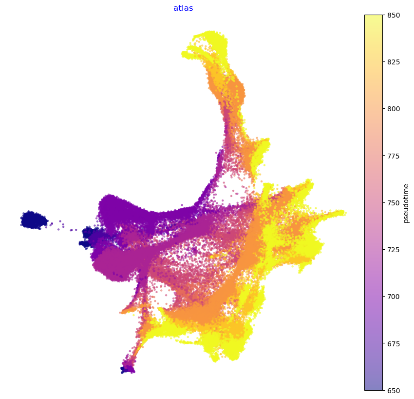
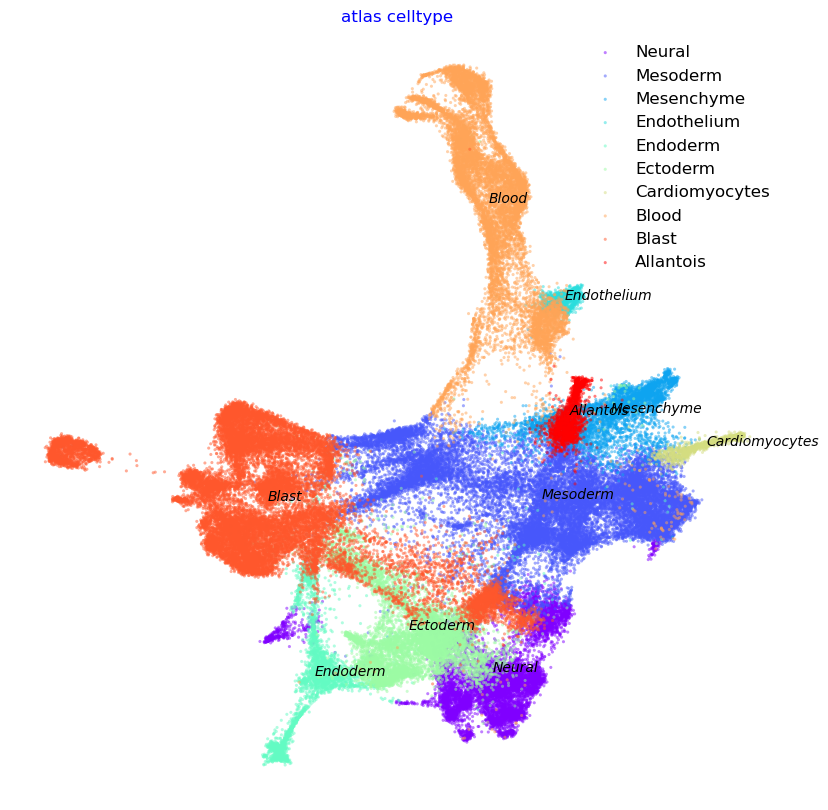
Take a look at the data using the stored Atlas single-cell embedding
We show the Atlas View (precomputed and saved here for convenience) colored by tissue type and gastrulation stage. Note that we have change the gastrulation time-stamps to numerical values. E.g. E6.5 becomes 650, E7.25 becoems 750 etc. Continue reading to see how the Atlas View is generated.
#plot the stored atlas embeddings by stage and cell type
print(f'{datetime.now()}\tStart plotting the saved via2 atlas embedding')
stage_label_numeric = [i for i in adata.obs['stage_num']]
cell_type_label = [i for i in     adata.obs['celltype']]

coarse_cell_type_label= [i for i in adata.obs['celltype_coarse']]
print('coarse cell_type', set(coarse_cell_type_label))
'''
#color by stage
f1, ax = via.plot_scatter(embedding=adata.obsm['X_Via2_atlas'] , labels=stage_label_numeric, cmap='plasma', s=5,
                          alpha=0.5, edgecolors='None',
                          title='atlas', text_labels=False)
f1.set_size_inches(10, 10)
'''

f2, ax = via.plot_scatter(embedding=adata.obsm['X_Via2_atlas'] , labels=coarse_cell_type_label, title='atlas coarse tissue type',
                          alpha=0.5, s=5)
f2.set_size_inches(10, 10)
2023-10-04 13:50:14.362904	Start plotting the saved via2 atlas embedding
coarse cell_type {'Endothelium', 'Cardiomyocytes', 'Blood', 'Mesenchyme', 'Blast', 'Mesoderm', 'Endoderm', 'Ectoderm', 'Allantois', 'Neural'}

Set parameters for Via 2.0
A quick note on how to (auto) set the root
group level user-defined suggestion: e.g.
root = ['Epiblast']The group level root assignment must correspond to a label that exists in the True-label parameter (must be passed inside a list).For autodetection based on rna-velocity root can be left as None. Since we will be using the velocity matrices (see below), Via 2.0 will suggest a list of likely root cell states that the user can decide to choose between. It is helpful to examine the top 5 suggested roots and choose the one that seems most reasonable. Note in the output that Via 2.0’s suggestions are almost all in the epibliast or Primitive streak state
A single cell index can also be passed e.g. [25], means the 25th cell will be used as a root.
Sequential Time-series labels
Set
time_series=Trueand pass the numerical time-series labels to Via using the parametertime_series_labels = stage_label_numericwhich accepts a list of length n_cells. The trajectory will be adjusted to reinforce edges based on temporal adjacency and optionally weed out edges that are between cells more thant_diff_stepapart.The number of sequential edges
knn_sequentialcan be used to emphasize adjacency in relation to edges between non-temporally adjacent edges.
Remark on Memory
In most cases of well connected population, higher memory (10-100) helps the root-to-fate pathway avoid detours into unrelated populations. For rare populations, or those without many precursor populations, it can be useful to lower memory to between 1-10 in order to allow for more exploration.
#set parameters for Via 2.0
memory=100 #this is a high memory value and will result in probabilistic pathways that avoid transitioning into unrelated cell populations
cluster_graph_pruning = 0.15 #level of pruning done on the cluster graph. higher number means less pruning (values can range from 0-3 standard deviations)
edgepruning_clustering_resolution = 0.15  # regulates number of clusters. Higher values means fewer clusters (values can range from 0-3 standard deviations)
random_seed = 42
knn = 30  # number of neighbors in the knn graph
knn_sequential = 15  # number of neighbors additionally created between sequentially adjacent time points
n_pcs = 30 # number of principal components
velo_weight = 0.5  # 0.7 #weight given to velocity based direction compared to pseudotime based direction
t_diff_step = 2 #edges extending between nodes that are more than 2 time steps apart will be removed (i.e. equal to 3 or more time steps apart)
root = ['Epiblast_13'] #for reproducibility, we set the root here. the group level root assignment must correspond to a label that exists in the True-label parameter (must be passed inside a list). For autodetection based on rna-velocity it can be left as None. A single cell index can also be passed e.g. [256], means the 256th cell will be used as a root. Since we will be using the velocity matrices (see below), Via 2.0 will suggest a list of likely root cell states that the user can decide to choose between. It is helpful to examine the top 5 suggested roots and choose the one that seems most reasonable. Note in the output that Via 2.0's suggestions are almost all in the epibliast or Primitive streak state
neighboring_terminal_states_threshold = 4
max_visual_outgoing_edges = 10#5 #used in differentiation flow chart plots
time_series = True

#get velocity and gene_matrices
subset = np.ones(adata.n_vars, bool)
subset &= np.array(adata.var["velocity_genes"].values, dtype=bool)
gene_matrix = np.asmatrix(adata.layers['Ms'][:, subset])  # None
velocity_matrix = adata.layers['velocity'][:, subset]  # None
cluster_celltype_label = [i for i in adata.obs['celltype_parc']]

#For reproducability we set the terminal states based on previous runs of Via 2.0 where the following cell fates were identified. This parameter can be left blank and a similar set of terminal states will be retrieved. This allows the user to control which suggested terminal states they are actually interested in or remove "duplicate" terminal states. The items in the list must correspond to items in the true_label list passed to Via 2.0.
user_defined_terminal_group_auto = ['Erythroid3_48',
                                    'Erythroid3_12', 'Erythroid3_55',
                                    'Haematoendothelial progenitors_26',
                                    'Haematoendothelial progenitors_42', 'Haematoendothelial progenitors_61',
                                    'Paraxial mesoderm_15', 'Paraxial mesoderm_19', 'Paraxial mesoderm_56',
                                    'Paraxial mesoderm_32', 'Cardiomyocytes_39', 'Intermediate mesoderm_6',
                                    'Intermediate mesoderm_8', 'ExE mesoderm_46',
                                    'Allantois_63', 'Mesenchyme_66', 'Mesenchyme_71', 'NMP_57', 'NMP_59', 'NMP_36',
                                    'NMP_54', 'Neural crest_69', 'Forebrain/Midbrain/Hindbrain_25',
                                    'Forebrain/Midbrain/Hindbrain_24',
                                    'Forebrain/Midbrain/Hindbrain_44', 'Forebrain/Midbrain/Hindbrain_25',
                                    'Paraxial mesoderm_56',
                                    'Visceral endoderm_41', 'Visceral endoderm_70',
                                    'Surface ectoderm_49', 'Surface ectoderm_50', ]
Initialize and Run the Via2.0
Optional: Predefined cluster labels and terminal cell fates
By default, Via will compute its own clusters and terminal cell fates. However, in some cases it may be desirable to provide pre-computed cluster groupings or set terminal cell fates. This can also be helfpul for reproducibility.
In the example below, we set the clusters to those that we have computed on a prior run of Via. labels = [list of numeric labels] of length n_cells.
We also set the cell fates to those precomputed by Via. user_defined_terminal_group = [list of cell fates that corresponding to items in true_label] This could also be provided as user_defined_terminal_cell=[list of cell indices corresponding to cell fates]
print(f'{datetime.now()}\tRun Via2.0')
parc_numeric_cluster_labels = [i for i in adata.obs['parc']]
parc_numeric_cluster_flat_array= np.asarray(parc_numeric_cluster_labels).flatten()
v0 = via.VIA(adata.obsm['X_pca'][:, 0:n_pcs], true_label= cluster_celltype_label, edgepruning_clustering_resolution=edgepruning_clustering_resolution,
             edgepruning_clustering_resolution_local=1, knn=knn, memory=memory, labels = parc_numeric_cluster_labels,
             cluster_graph_pruning=cluster_graph_pruning,
             neighboring_terminal_states_threshold=neighboring_terminal_states_threshold,
             too_big_factor=0.3, resolution_parameter=1,
             root_user=root, dataset='group', random_seed=random_seed,
             is_coarse=True, preserve_disconnected=False, pseudotime_threshold_TS=40, x_lazy=0.99,
             do_gaussian_kernel_edgeweights=False,
             alpha_teleport=0.99, edgebundle_pruning=cluster_graph_pruning, edgebundle_pruning_twice=False,
             velo_weight=velo_weight, velocity_matrix=velocity_matrix, gene_matrix=gene_matrix,
             time_series=time_series, time_series_labels=stage_label_numeric, knn_sequential=knn_sequential,
             knn_sequential_reverse=knn_sequential, t_diff_step=t_diff_step, RW2_mode=False,

             user_defined_terminal_group=user_defined_terminal_group_auto,
             max_visual_outgoing_edges=max_visual_outgoing_edges)
v0.run_VIA()
print(f'{datetime.now()}\tEnd Via2.0 computation')
2023-10-04 14:08:43.821979	Run Via2.0
2023-10-04 14:08:44.183992	Running VIA over input data of 89267 (samples) x 30 (features)
2023-10-04 14:08:44.184090	Knngraph has 30 neighbors
2023-10-04 14:09:06.782957	Using time series information to guide knn graph construction
2023-10-04 14:09:06.800664	Time series ordered set [650, 675, 700, 725, 750, 775, 800, 825, 850]
2023-10-04 14:09:46.819205	Shape neighbors (89267, 30) and sequential neighbors (89267, 30)
2023-10-04 14:09:46.856059	Shape augmented neighbors (89267, 60)
2023-10-04 14:09:46.877363	Actual average allowable time difference between nodes is 50.0
2023-10-04 14:10:16.996644	Finished global pruning of 30-knn graph used for clustering at level of 0.15. Kept 49.4 % of edges.
2023-10-04 14:10:17.115905	Number of connected components used for clustergraph  is 1
2023-10-04 14:10:35.514207	Using predfined labels provided by user (this must be provided as an array)
2023-10-04 14:10:35.514325	Making cluster graph. Global cluster graph pruning level: 0.15
2023-10-04 14:10:36.551417	Graph has 1 connected components before pruning
2023-10-04 14:10:36.559069	Graph has 1 connected components after pruning
2023-10-04 14:10:36.559384	Graph has 1 connected components after reconnecting
2023-10-04 14:10:36.560546	23.8% links trimmed from local pruning relative to start
2023-10-04 14:10:36.560574	82.4% links trimmed from global pruning relative to start
size velocity matrix 89267 (89267, 1784)
2023-10-04 14:10:41.604510	Looking for initial states
2023-10-04 14:10:41.613896	Stationary distribution normed [0.008 0.012 0.022 0.007 0.006 0.027 0.019 0.035 0.032 0.014 0.015 0.005
 0.004 0.002 0.011 0.014 0.057 0.009 0.017 0.014 0.005 0.011 0.03  0.01
 0.007 0.008 0.014 0.014 0.013 0.028 0.01  0.022 0.015 0.008 0.012 0.019
 0.027 0.027 0.033 0.009 0.014 0.017 0.012 0.007 0.009 0.019 0.009 0.005
 0.003 0.009 0.009 0.01  0.004 0.003 0.018 0.003 0.009 0.008 0.005 0.008
 0.011 0.009 0.011 0.011 0.007 0.017 0.017 0.009 0.003 0.003 0.015 0.017
 0.013 0.026]
2023-10-04 14:10:41.614671	Top 5 candidates for root: [13 55 69 68 53 48 52 12 58 11] with stationary prob (%) [0.204 0.252 0.271 0.28  0.292 0.297 0.356 0.364 0.456 0.456]
2023-10-04 14:10:41.614990	Top 5 candidates for terminal: [16  7 38  8 22]
cell type of suggested roots: ['Epiblast_58', 'Primitive Streak_58', 'Visceral endoderm_41', 'Primitive Streak_58', 'Epiblast_58', 'Epiblast_58', 'Primitive Streak_58', 'Epiblast_58', 'Epiblast_58', 'Primitive Streak_58']
cell stage of suggested roots: [650, 650, 650, 650, 650, 650, 650, 650, 650, 650]
2023-10-04 14:10:41.629833	component number 0 out of  [0]
2023-10-04 14:10:41.840290	group root method
2023-10-04 14:10:41.841040	for component 0, the root is Epiblast_13 and ri Epiblast_13
cluster 0 has majority Epiblast_0
cluster 1 has majority Nascent mesoderm_1
cluster 2 has majority Rostral neurectoderm_2
cluster 3 has majority Primitive Streak_3
cluster 4 has majority Epiblast_4
cluster 5 has majority Forebrain/Midbrain/Hindbrain_5
cluster 6 has majority Intermediate mesoderm_6
cluster 7 has majority Paraxial mesoderm_7
cluster 8 has majority Intermediate mesoderm_8
cluster 9 has majority Rostral neurectoderm_9
cluster 10 has majority Erythroid1_10
cluster 11 has majority Epiblast_11
cluster 12 has majority Erythroid3_12
cluster 13 has majority Epiblast_13
2023-10-04 14:10:42.840939	New root is 13 and majority Epiblast_13
cluster 14 has majority Nascent mesoderm_14
cluster 15 has majority Paraxial mesoderm_15
cluster 16 has majority Mesenchyme_16
cluster 17 has majority Rostral neurectoderm_17
cluster 18 has majority Erythroid1_18
cluster 19 has majority Paraxial mesoderm_19
cluster 20 has majority Nascent mesoderm_20
cluster 21 has majority Blood progenitors 2_21
cluster 22 has majority Paraxial mesoderm_22
cluster 23 has majority Epiblast_23
cluster 24 has majority Forebrain/Midbrain/Hindbrain_24
cluster 25 has majority Forebrain/Midbrain/Hindbrain_25
cluster 26 has majority Haematoendothelial progenitors_26
cluster 27 has majority Epiblast_27
cluster 28 has majority Mesenchyme_28
cluster 29 has majority Gut_29
cluster 30 has majority Erythroid1_30
cluster 31 has majority Surface ectoderm_31
cluster 32 has majority Paraxial mesoderm_32
cluster 33 has majority Rostral neurectoderm_33
cluster 34 has majority Rostral neurectoderm_34
cluster 35 has majority Forebrain/Midbrain/Hindbrain_35
cluster 36 has majority NMP_36
cluster 37 has majority Intermediate mesoderm_37
cluster 38 has majority Allantois_38
cluster 39 has majority Cardiomyocytes_39
cluster 40 has majority Epiblast_40
cluster 41 has majority Visceral endoderm_41
cluster 42 has majority Haematoendothelial progenitors_42
cluster 43 has majority Anterior Primitive Streak_43
cluster 44 has majority Forebrain/Midbrain/Hindbrain_44
cluster 45 has majority Rostral neurectoderm_45
cluster 46 has majority ExE mesoderm_46
cluster 47 has majority Epiblast_47
cluster 48 has majority Erythroid3_48
cluster 49 has majority Surface ectoderm_49
cluster 50 has majority Surface ectoderm_50
cluster 51 has majority Erythroid1_51
cluster 52 has majority Rostral neurectoderm_52
cluster 53 has majority Notochord_53
cluster 54 has majority NMP_54
cluster 55 has majority Erythroid3_55
cluster 56 has majority Paraxial mesoderm_56
cluster 57 has majority NMP_57
cluster 58 has majority Epiblast_58
cluster 59 has majority NMP_59
cluster 60 has majority Surface ectoderm_60
cluster 61 has majority Haematoendothelial progenitors_61
cluster 62 has majority Erythroid1_62
cluster 63 has majority Allantois_63
cluster 64 has majority Haematoendothelial progenitors_64
cluster 65 has majority Gut_65
cluster 66 has majority Mesenchyme_66
cluster 67 has majority Mesenchyme_67
cluster 68 has majority PGC_68
cluster 69 has majority Neural crest_69
cluster 70 has majority Visceral endoderm_70
cluster 71 has majority Mesenchyme_71
cluster 72 has majority Allantois_72
cluster 73 has majority Mesenchyme_73
2023-10-04 14:10:43.534093	Computing lazy-teleporting expected hitting times
2023-10-04 14:10:47.653021	 ended all multiprocesses, will retrieve and reshape
try rw2 hitting times setup
start computing walks with rw2 method
g.indptr.size, 75
/home/user/anaconda3/envs/Via2Env_py10/lib/python3.10/site-packages/pecanpy/graph.py:90: UserWarning: WARNING: Implicitly set node IDs to the canonical node ordering due to missing IDs field in the raw CSR npz file. This warning message can be suppressed by setting implicit_ids to True in the read_npz function call, or by setting the --implicit_ids flag in the CLI
  warnings.warn(
memory for rw2 hittings times  2. Using rw2 based pt
do scaling of pt
2023-10-04 14:10:55.012227	Terminal cluster list based on user defined cells/groups: [('Erythroid3_48', 48), ('Erythroid3_12', 12), ('Erythroid3_55', 55), ('Haematoendothelial progenitors_26', 26), ('Haematoendothelial progenitors_42', 42), ('Haematoendothelial progenitors_61', 61), ('Paraxial mesoderm_15', 15), ('Paraxial mesoderm_19', 19), ('Paraxial mesoderm_56', 56), ('Paraxial mesoderm_32', 32), ('Cardiomyocytes_39', 39), ('Intermediate mesoderm_6', 6), ('Intermediate mesoderm_8', 8), ('ExE mesoderm_46', 46), ('Allantois_63', 63), ('Mesenchyme_66', 66), ('Mesenchyme_71', 71), ('NMP_57', 57), ('NMP_59', 59), ('NMP_36', 36), ('NMP_54', 54), ('Neural crest_69', 69), ('Forebrain/Midbrain/Hindbrain_25', 25), ('Forebrain/Midbrain/Hindbrain_24', 24), ('Forebrain/Midbrain/Hindbrain_44', 44), ('Visceral endoderm_41', 41), ('Visceral endoderm_70', 70), ('Surface ectoderm_49', 49), ('Surface ectoderm_50', 50)]
2023-10-04 14:10:55.012836	Terminal clusters corresponding to unique lineages in this component are [48, 12, 55, 26, 42, 61, 15, 19, 56, 32, 39, 6, 8, 46, 63, 66, 71, 57, 59, 36, 54, 69, 25, 24, 44, 41, 70, 49, 50]
TESTING rw2_lineage probability at memory 100
testing rw2 lineage probability at memory 100
g.indptr.size, 75
/home/user/anaconda3/envs/Via2Env_py10/lib/python3.10/site-packages/pecanpy/graph.py:90: UserWarning: WARNING: Implicitly set node IDs to the canonical node ordering due to missing IDs field in the raw CSR npz file. This warning message can be suppressed by setting implicit_ids to True in the read_npz function call, or by setting the --implicit_ids flag in the CLI
  warnings.warn(
2023-10-04 14:10:59.943211	 Cluster or terminal cell fate 48 is reached 45.0 times
2023-10-04 14:11:00.206447	 Cluster or terminal cell fate 12 is reached 41.0 times
2023-10-04 14:11:00.488101	 Cluster or terminal cell fate 55 is reached 22.0 times
2023-10-04 14:11:00.762313	 Cluster or terminal cell fate 26 is reached 35.0 times
2023-10-04 14:11:01.037768	 Cluster or terminal cell fate 42 is reached 40.0 times
2023-10-04 14:11:01.303138	 Cluster or terminal cell fate 61 is reached 36.0 times
2023-10-04 14:11:01.582438	 Cluster or terminal cell fate 15 is reached 29.0 times
2023-10-04 14:11:01.853243	 Cluster or terminal cell fate 19 is reached 22.0 times
2023-10-04 14:11:02.147883	 Cluster or terminal cell fate 56 is reached 2.0 times
2023-10-04 14:11:02.345118	 Cluster or terminal cell fate 32 is reached 28.0 times
2023-10-04 14:11:02.598388	 Cluster or terminal cell fate 39 is reached 34.0 times
2023-10-04 14:11:02.845540	 Cluster or terminal cell fate 6 is reached 79.0 times
2023-10-04 14:11:03.083305	 Cluster or terminal cell fate 8 is reached 94.0 times
2023-10-04 14:11:03.366535	 Cluster or terminal cell fate 46 is reached 33.0 times
2023-10-04 14:11:03.637805	 Cluster or terminal cell fate 63 is reached 103.0 times
2023-10-04 14:11:03.900672	 Cluster or terminal cell fate 66 is reached 11.0 times
2023-10-04 14:11:04.172938	 Cluster or terminal cell fate 71 is reached 14.0 times
2023-10-04 14:11:04.431325	 Cluster or terminal cell fate 57 is reached 22.0 times
2023-10-04 14:11:04.707598	 Cluster or terminal cell fate 59 is reached 61.0 times
2023-10-04 14:11:04.982094	 Cluster or terminal cell fate 36 is reached 72.0 times
2023-10-04 14:11:05.258765	 Cluster or terminal cell fate 54 is reached 59.0 times
2023-10-04 14:11:05.526827	 Cluster or terminal cell fate 69 is reached 39.0 times
2023-10-04 14:11:05.805750	 Cluster or terminal cell fate 25 is reached 74.0 times
2023-10-04 14:11:06.100490	 Cluster or terminal cell fate 24 is reached 23.0 times
2023-10-04 14:11:06.374214	 Cluster or terminal cell fate 44 is reached 42.0 times
2023-10-04 14:11:06.643444	 Cluster or terminal cell fate 41 is reached 26.0 times
2023-10-04 14:11:06.897360	 Cluster or terminal cell fate 70 is reached 20.0 times
2023-10-04 14:11:07.149146	 Cluster or terminal cell fate 49 is reached 181.0 times
2023-10-04 14:11:07.400434	 Cluster or terminal cell fate 50 is reached 173.0 times
2023-10-04 14:11:08.403681	There are (29) terminal clusters corresponding to unique lineages {48: 'Erythroid3_48', 12: 'Erythroid3_12', 55: 'Erythroid3_55', 26: 'Haematoendothelial progenitors_26', 42: 'Haematoendothelial progenitors_42', 61: 'Haematoendothelial progenitors_61', 15: 'Paraxial mesoderm_15', 19: 'Paraxial mesoderm_19', 56: 'Paraxial mesoderm_56', 32: 'Paraxial mesoderm_32', 39: 'Cardiomyocytes_39', 6: 'Intermediate mesoderm_6', 8: 'Intermediate mesoderm_8', 46: 'ExE mesoderm_46', 63: 'Allantois_63', 66: 'Mesenchyme_66', 71: 'Mesenchyme_71', 57: 'NMP_57', 59: 'NMP_59', 36: 'NMP_36', 54: 'NMP_54', 69: 'Neural crest_69', 25: 'Forebrain/Midbrain/Hindbrain_25', 24: 'Forebrain/Midbrain/Hindbrain_24', 44: 'Forebrain/Midbrain/Hindbrain_44', 41: 'Visceral endoderm_41', 70: 'Visceral endoderm_70', 49: 'Surface ectoderm_49', 50: 'Surface ectoderm_50'}
2023-10-04 14:11:08.403829	Begin projection of pseudotime and lineage likelihood
2023-10-04 14:11:13.990792	Start reading data
2023-10-04 14:11:13.990883	Correlation of Via pseudotime with developmental stage 84.92 %
2023-10-04 14:11:14.042484	Transition matrix with weight of 0.5 on RNA velocity
2023-10-04 14:11:14.042955	Cluster graph layout based on forward biasing
2023-10-04 14:11:14.059714	Starting make edgebundle viagraph...
2023-10-04 14:11:14.059769	Make via clustergraph edgebundle
2023-10-04 14:11:14.814543	Hammer dims: Nodes shape: (74, 2) Edges shape: (446, 3)
2023-10-04 14:11:14.816250	Graph has 1 connected components before pruning
2023-10-04 14:11:14.821502	Graph has 4 connected components after pruning
2023-10-04 14:11:14.827656	Graph has 1 connected components after reconnecting
2023-10-04 14:11:14.828729	1.8% links trimmed from local pruning relative to start
2023-10-04 14:11:14.828759	63.2% links trimmed from global pruning relative to start
/home/user/anaconda3/envs/Via2Env_py10/lib/python3.10/site-packages/scipy/sparse/_index.py:103: SparseEfficiencyWarning: Changing the sparsity structure of a csr_matrix is expensive. lil_matrix is more efficient.
  self._set_intXint(row, col, x.flat[0])
2023-10-04 14:11:15.208715	Time elapsed 132.3 seconds
2023-10-04 14:11:15.209000	End Via2.0 computation
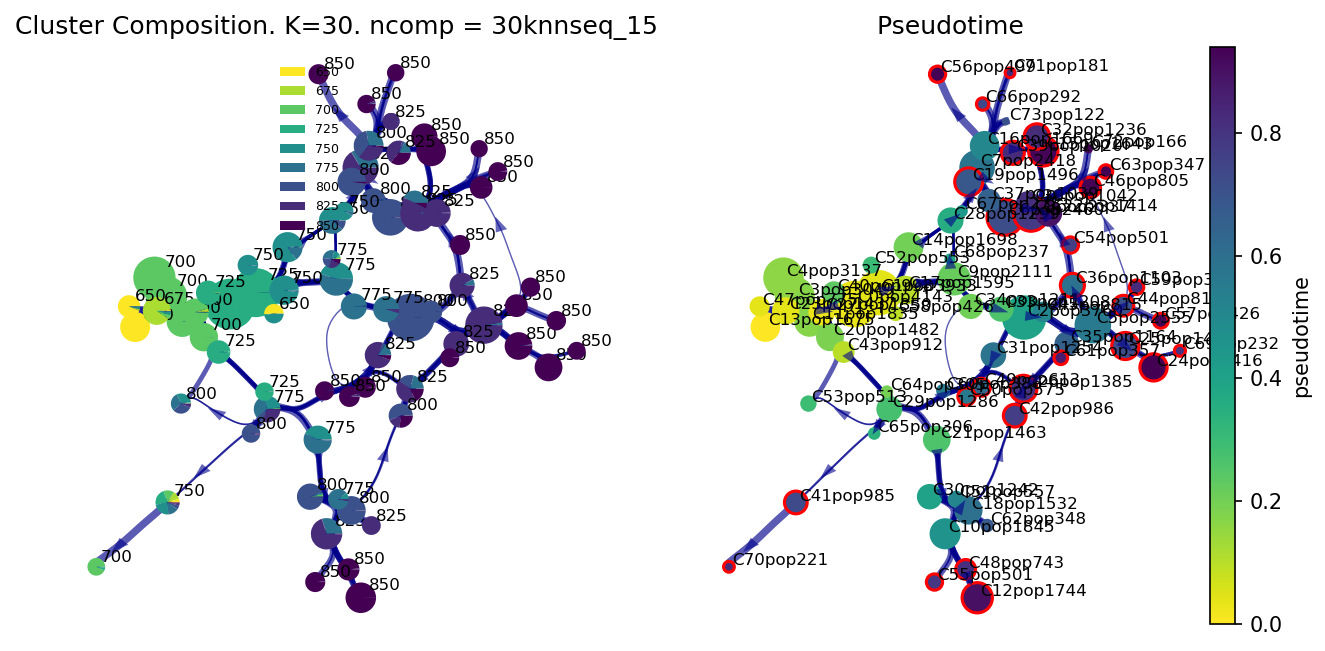
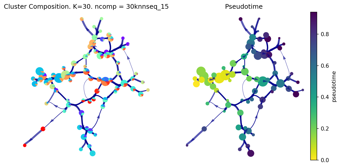
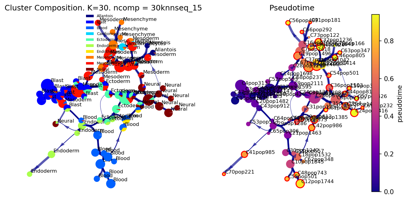
Plot Via2.0 cluster graph
Examples showing how to control the colormaps, labeling and choice of attribute to plot on the viagraph
print(f'{datetime.now()}\tPlot Via2.0 cluster graph')

f, ax, ax1=via.plot_piechart_viagraph(via_object=v0, cmap_piechart='viridis_r', cmap='viridis_r',                        reference_labels=stage_label_numeric, headwidth_arrow=0.4,
                        highlight_terminal_clusters=True)
f.set_size_inches(10, 5)
f, ax, ax1=via.plot_piechart_viagraph(via_object=v0, headwidth_arrow=0.4, show_legend=False, ax_text=False, pie_size_scale=0.6,
                        highlight_terminal_clusters=False, size_node_notpiechart=0.8)
f.set_size_inches(10, 5)
f, ax, ax1= via.plot_piechart_viagraph(via_object=v0, cmap_piechart='jet', cmap='plasma',
                        reference_labels=coarse_cell_type_label, headwidth_arrow=0.4,
                        highlight_terminal_clusters=True,size_node_notpiechart=0.8)
f.set_size_inches(10, 5)
2023-10-04 14:18:30.361275 Plot Via2.0 cluster graph
/home/user/PycharmProjects/Via2_May2023_py310/plotting_via.py:3092: UserWarning: No data for colormapping provided via 'c'. Parameters 'cmap' will be ignored
  sct = ax.scatter(node_pos[:, 0], node_pos[:, 1],
/home/user/PycharmProjects/Via2_May2023_py310/plotting_via.py:3092: UserWarning: No data for colormapping provided via 'c'. Parameters 'cmap' will be ignored
  sct = ax.scatter(node_pos[:, 0], node_pos[:, 1],
/home/user/PycharmProjects/Via2_May2023_py310/plotting_via.py:3092: UserWarning: No data for colormapping provided via 'c'. Parameters 'cmap' will be ignored
  sct = ax.scatter(node_pos[:, 0], node_pos[:, 1],
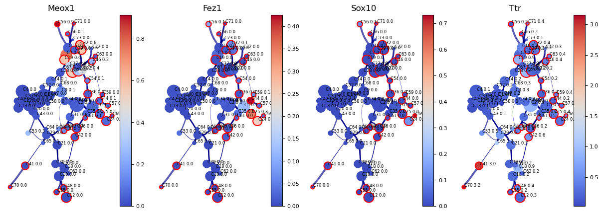
genes=['Meox1','Fez1','Sox10','Ttr']
df_genes_sc = pd.DataFrame(adata[:, genes].X.todense(), columns=genes)
fig, axs=via.plot_viagraph(via_object=v0, df_genes=df_genes_sc, gene_list=genes)#, label_text=False)
fig.set_size_inches(15,5)
Compute Atlas single-cell embedding
We transfer the properties of the trajectory infused viagraph and the single-cell temporally adjusted graph to generate an embedding that visually conveys the structure of the trajectory and can be used as the basis of the Atlas View (described farther down)
If you want to plot the pre-computed atlas embedding set compute_atlas_embedding = False, otherwise compute the atlas embedding. We can then plot the atlas view based on cell type or other attributes.
print(f'{datetime.now()}\tStart Atlas embedding computation')
compute_atlas_embedding = True
if compute_atlas_embedding:
    atlas_embedding = via.via_atlas_emb(via_object=v0, init_pos='via', min_dist=0.2)
else: atlas_embedding = embedding=adata.obsm['X_Via2_atlas']

print(f'{datetime.now()}\tPlot Atlas Embedding')
f1, ax = via.plot_scatter(embedding=atlas_embedding, labels=stage_label_numeric, cmap='plasma', s=5,
                          alpha=0.5, edgecolors='None',
                          title='atlas', text_labels=False)
f1.set_size_inches(10, 10)

f2, ax = via.plot_scatter(embedding=atlas_embedding, labels=coarse_cell_type_label, title='atlas celltype',
                          alpha=0.5, s=5)
f2.set_size_inches(10, 10)
#plt.show()
No artists with labels found to put in legend. Note that artists whose label start with an underscore are ignored when legend() is called with no argument.
2023-09-20 10:57:23.986672	Start Atlas embedding computation
2023-09-20 10:57:23.987906	Plot Atlas Embedding
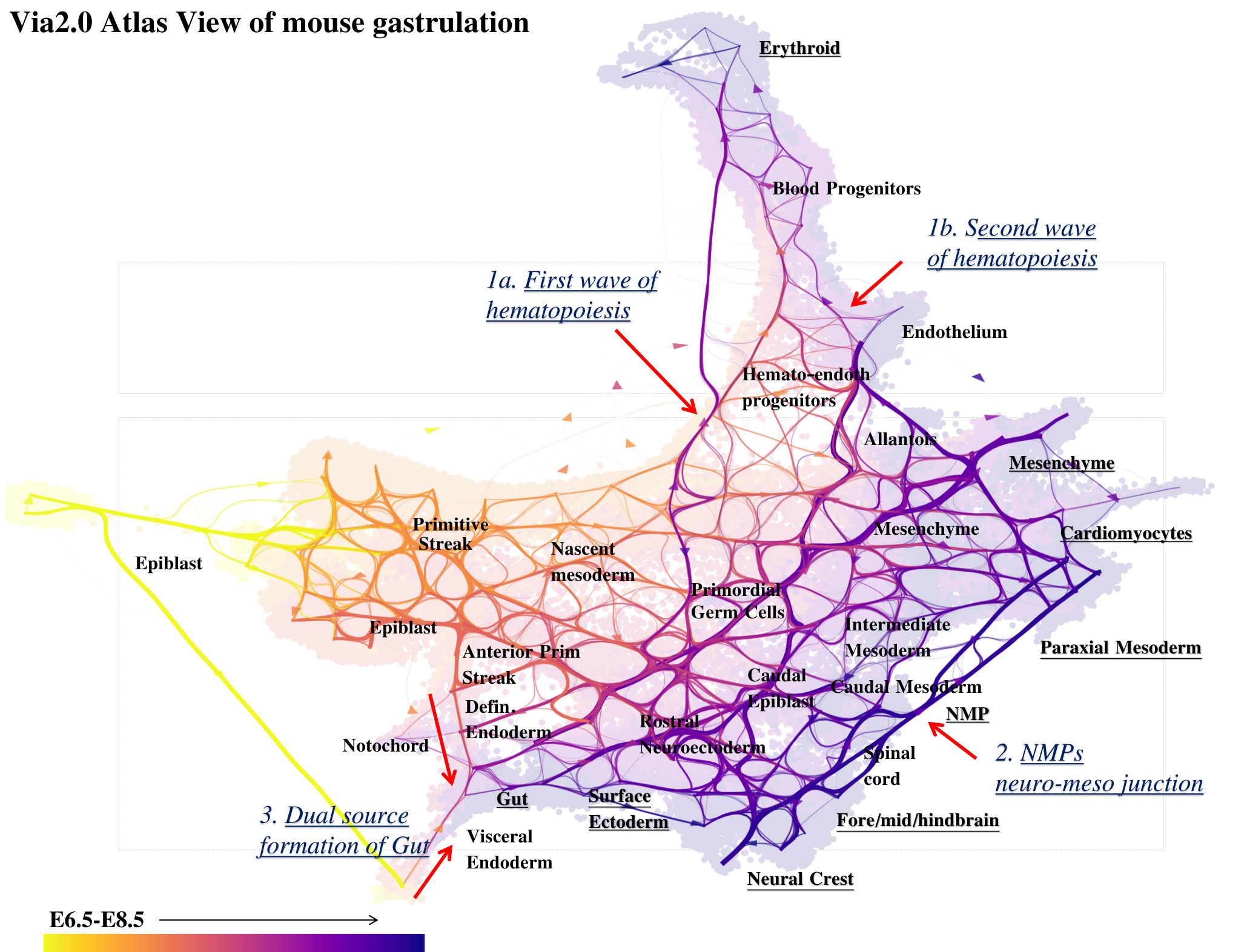
The Atlas View
Now we look at how to construct the atlas view which combines the single-cell spatial layout with a high-resoulution view of the edge connectivity (potential pathways).
If you want more control then consider running the edge construction step shown in STEP 1
You can skip STEP 1 and directly call plot_atlas_view() in STEP 2 and set a parameter n_milestones to the desired granularity. This parameter is o/w autoset based on data.
print(f'{datetime.now()}\tCreate edgebundle')
# STEP 1
decay = 0.6  # increasing decay increasing merging of edges
i_bw = 0.02  # increasing bw increases merging of edges
global_visual_pruning = 0.6  # increasing this retains more edges
v0.embedding = atlas_embedding #pass the embedding we computed into the Via object

import random
pseudorand = random.randint(0, 1000)
n_milestones = 150
hammerbundle_dict = via.make_edgebundle_milestone(via_object=v0, n_milestones=n_milestones, decay=decay,
                                                  initial_bandwidth=i_bw, global_visual_pruning=global_visual_pruning,
                                                  sc_labels_numeric=stage_label_numeric)
v0.hammerbundle_milestone_dict = hammerbundle_dict  # make the hmbd and assign it to the via_object. this can then be used for all plots without having to recompute it
print(f'{datetime.now()}\tPlot edgebundle')
# STEP 2
dict_coarse = {'Neural': 2.5, 'Mesoderm': 3.5, 'neural_crest': 4.5, 'Mesenchyme': 5,
                   'Endothelium': 7, 'Endoderm': 1.25,
                   'Ectoderm': 2, 'Cardiomyocytes': 6, 'Blood': 8, 'Blast': 0,'Allantois':4}
fig, ax = via.plot_atlas_view(via_object=v0, decay=decay, initial_bandwidth=i_bw, add_sc_embedding=True,
                               sc_labels_expression=[dict_coarse[coarse_cell_type_label[i]] for i in
                                                     range(len(v0.labels))], sc_scatter_alpha=0.01,
                               scatter_size_sc_embedding=5,
                               linewidth_bundle=4, alpha_bundle_factor=1.5, headwidth_bundle=0.2,
                               cmap='rainbow', facecolor='white', size_scatter=1, alpha_scatter=0.1,
                               global_visual_pruning=global_visual_pruning,
                               scale_scatter_size_pop=True, fontsize_labels=16,
                               extra_title_text='EStage decay:' + str(decay) + ' bw:' + str(
                                   i_bw) + 'globalVisPruning:' + str(global_visual_pruning),
                               text_labels=False, sc_labels=cell_type_label, use_sc_labels_sequential_for_direction=True)
fig.set_size_inches(35, 25)

'''
fig, ax = via.plot_atlas_view(via_object=v0, decay=decay, initial_bandwidth=i_bw, add_sc_embedding=True, sc_labels_expression=stage_label_numeric,sc_scatter_alpha=0.15,scatter_size_sc_embedding=10,
                     linewidth_bundle=3, alpha_bundle_factor=1.5, headwidth_bundle=0.2,
                     cmap='plasma_r', facecolor='white', size_scatter=1, alpha_scatter=0.1,  global_visual_pruning=global_visual_pruning,
                     scale_scatter_size_pop=True, fontsize_labels=16,
                     extra_title_text='EStage decay:' + str(decay) + ' bw:' + str(i_bw)+'globalVisPruning:'+str(global_visual_pruning),
                     text_labels=False, sc_labels=cell_type_label, use_sc_labels_sequential_for_direction=True)
fig.set_size_inches(35, 25)
plt.show()
'''
2023-09-21 08:02:37.438382	Plot edgebundle
inside add sc embedding second if
"\nfig, ax = via.plot_edge_bundle(via_object=v0, decay=decay, initial_bandwidth=i_bw, add_sc_embedding=True, sc_labels_expression=stage_label_numeric,sc_scatter_alpha=0.15,scatter_size_sc_embedding=10,\n linewidth_bundle=3, alpha_bundle_factor=1.5, headwidth_bundle=0.2,\n cmap='plasma_r', facecolor='white', size_scatter=1, alpha_scatter=0.1, global_visual_pruning=global_visual_pruning,\n scale_scatter_size_pop=True, fontsize_labels=16,\n extra_title_text='EStage decay:' + str(decay) + ' bw:' + str(i_bw)+'globalVisPruning:'+str(global_visual_pruning),\n text_labels=False, sc_labels=cell_type_label, use_sc_labels_sequential_for_direction=True)\nfig.set_size_inches(35, 25)\nplt.show()\n"
Plot single-cell lineage probabilities
Memory
The lineage probability pathways below are computed based on a memory parameter value of 100 (set when we initialized Via), this is a high degree of memory. Sometimes a very high memory can prevent rarer population from being reached, depending on the connectivity of the network. You can always try lowering the value to e.g. 10 or 50.
If you run Via at memory=1 (the no memory case), and then plot the lineage probability pathways and gene trends, you will notice that many of the pathways are diffuse (migrating into unrelated cell populations) and the gene trends can overlap and not be very discriminative.
print(f'{datetime.now()}\tPlot single-cell lineage probabilities')

select_terminal_clusters =  [15, 69, 24, 71, 50, 36]
fig, ax = via.plot_atlas_view(via_object=v0, lineage_pathway=select_terminal_clusters, linewidth_bundle=4, alpha_bundle_factor=5, headwidth_bundle=0.4,
                                           size_scatter=0.05, alpha_scatter=0.3, sc_scatter_size=3, sc_scatter_alpha=0.3,
                                           use_sc_labels_sequential_for_direction=True)
fig.suptitle('lineage probabilities', fontsize=14)
fig.set_size_inches(25, 15)
2023-09-21 07:44:18.819316	Plot single-cell lineage probabilities
location of 15 is at [6] and 6
location of 69 is at [21] and 21
location of 24 is at [23] and 23
location of 71 is at [16] and 16
location of 50 is at [28] and 28
location of 36 is at [19] and 19
Plot gene trends
Memory
The gene trends use the lineage probabilities computed at a memory parameter value of 100, this is a high degree of memory which means the gene trends have higher specificity to their respective gene markers.
If you run Via at memory=1 (the no memory case), and then plot the lineage probability pathways and gene trends, you will notice that many of the pathways are diffuse (migrating into unrelated cell populations) and the gene trends can overlap and not be very discriminative.
genes=['Meox1','Fez1','Sox10','Ttr']
df_genes_sc = pd.DataFrame(adata[:, genes].X.todense(), columns=genes)

select_terminal_clusters = [15, 69, 44, 50]
spline_order = 3
n_splines = 5
fig, axs= via.get_gene_expression(via_object=v0, gene_exp=df_genes_sc, marker_genes=genes,
                        marker_lineages=select_terminal_clusters,  # 56,50,25
                        n_splines=n_splines, spline_order=spline_order, cmap='Accent')
print(memory,'q_memory')
plt.suptitle('Accent q_memory:' + str(memory))
fig.set_size_inches(10, 3)
100 q_memory
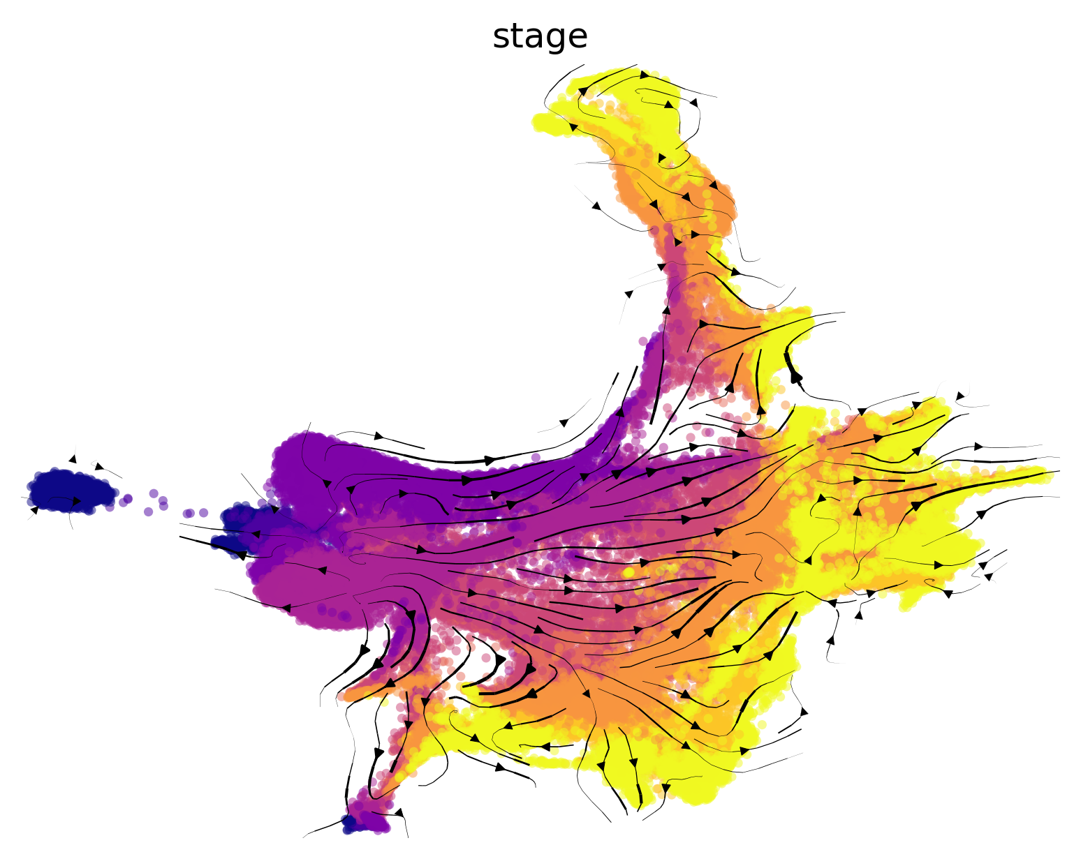
Plot stream plot using hybrid pseudotime-RNAvelocity based directionality
Using a combination of pseudotime and rna-velocity ensures biologically meaningful directionality
print(f'{datetime.now()}\tPlot stream plot')
via.via_streamplot(v0, embedding=atlas_embedding, scatter_size=10, scatter_alpha=0.5, marker_edgewidth=0.01, density_stream=2,
                   density_grid=1, smooth_transition=2, smooth_grid=0.5,  title='stage', labels=stage_label_numeric, cmap='plasma')
plt.show()
2023-09-20 14:53:34.466470 Plot stream plot
/home/user/anaconda3/envs/Via2Env_py10/lib/python3.10/site-packages/scipy/sparse/_index.py:146: SparseEfficiencyWarning: Changing the sparsity structure of a csr_matrix is expensive. lil_matrix is more efficient.
  self._set_arrayXarray(i, j, x)
/home/user/PycharmProjects/Via2_May2023_py310/core_working_rw2.py:1325: RuntimeWarning: divide by zero encountered in divide
  T = T.multiply(csr_matrix(1.0 / np.abs(T).sum(1)))  # rows sum to one
/home/user/PycharmProjects/Via2_May2023_py310/core_working_rw2.py:1349: RuntimeWarning: invalid value encountered in divide
  dX /= l2_norm(dX)[:, None]
/home/user/PycharmProjects/Via2_May2023_py310/core_working_rw2.py:1356: RuntimeWarning: Mean of empty slice.
  V_emb[i] = probs.dot(dX) - probs.mean() * dX.sum(0)
/home/user/anaconda3/envs/Via2Env_py10/lib/python3.10/site-packages/numpy/core/_methods.py:192: RuntimeWarning: invalid value encountered in scalar divide
  ret = ret.dtype.type(ret / rcount)