scRNA-seq Human Hematopoiesis
This notebook uses VIA to interpret the CD34 Hematopoiesis dataset (Setty et al.,2019)
import pyVIA.core as via
import pyVIA.datasets_via as   datasets
import pandas as pd
import scanpy as sc

import matplotlib.pyplot as plt
import warnings
warnings.filterwarnings('ignore')
Load data from directory
We use annotations given by SingleR which uses Novershtern Hematopoietic cell data as the reference. These are in line with the annotations given by Setty et al., 2019 but offer a slightly more granular annotation.
adata = datasets.scRNA_hematopoiesis()
sc.tl.pca(adata, svd_solver='arpack', n_comps=200)
tsnem = adata.obsm['tsne']
adata
Cell type CMP has  968 cells
Cell type PRE_B3 has  2 cells
Cell type B_a4 has  8 cells
Cell type pDC has  204 cells
Cell type HSC2 has  10 cells
Cell type GRAN1 has  3 cells
Cell type Nka3 has  5 cells
Cell type EOS2 has  3 cells
Cell type MONO1 has  186 cells
Cell type B_a1 has  27 cells
Cell type ERY3 has  104 cells
Cell type ERY1 has  773 cells
Cell type HSC1 has  2365 cells
Cell type MONO2 has  35 cells
Cell type ERY2 has  40 cells
Cell type mDC (cDC) has  96 cells
Cell type B_a2 has  1 cells
Cell type BASO1 has  2 cells
Cell type ERY4 has  53 cells
Cell type MEP has  339 cells
Cell type PRE_B2 has  515 cells
Cell type TCEL7 has  1 cells
Cell type GMP has  28 cells
Cell type MEGA1 has  12 cells
AnnData object with n_obs × n_vars = 5780 × 14651
    obs: 'clusters', 'palantir_pseudotime', 'palantir_diff_potential', 'label'
    uns: 'cluster_colors', 'ct_colors', 'palantir_branch_probs_cell_types', 'pca'
    obsm: 'tsne', 'MAGIC_imputed_data', 'palantir_branch_probs', 'X_pca'
    varm: 'PCs'
User’s choice of embedding
Three embedding exmaples: TSNE, UMAP, and PHATE Alternatively allow via.VIA() to compute an embedding using the underlying graph by setting: do_embedding = True AND embedding_type = ‘via-umap’ OR ‘via-mds’
# TSNE - same as the embedding used in the original Setty et al., publication
embedding = adata.obsm['tsne']

# # UMAP
# ncomp = 30
# embedding = umap.UMAP().fit_transform(adata.obsm['X_pca'][:, 0:ncomp])

# # PHATE
# ncomp = 30
# phate_op = phate.PHATE()
# embedding = phate_op.fit_transform(adata.obsm['X_pca'][:, 0:ncomp])
Run VIA
Key Parameters:
knn
root_user (root index of type int/ or celltype label of type string)
edgepruning_clustering_resolution (lower number means smaller (and more) clusters) typical range 0-1
memory (higher value means more focused search pathways to cell fates) typical range 2-50
cluster_graph_pruning (lower number means fewer edges) typical range 0-1
dataset (relates to the root_user parameter. if the root is an index, the leave as dataset =’’. If the root is a celltype label found in true_label paramters, then dataset=’group’)
ncomps=80
knn=30
v0_random_seed=4
root_user = [4823] #the index of a cell belonging to the HSC cell type
memory = 10
dataset = ''

'''
#NOTE1, if you decide to choose a cell type as a root, then you need to set the dataset as 'group'
#root_user=['HSC1']
#dataset = 'group'# 'humanCD34'
#NOTE2, if rna-velocity is available, considering using it to compute the root automatically- see RNA velocity tutorial
'''

v0 = via.VIA(data=adata.obsm['X_pca'][:, 0:ncomps], true_label=adata.obs['label'],
             edgepruning_clustering_resolution=0.15, cluster_graph_pruning=0.15,
             knn=knn,  root_user=root_user, resolution_parameter=1.5,
             dataset=dataset, random_seed=v0_random_seed, memory=memory)#, do_compute_embedding=True, embedding_type='via-atlas')

v0.run_VIA()

#NOTE2: if you want to pre-specify terminal states you can do so by a list of group-level names corresponding to true-labels OR by a list of single cell indices
#E.G. user_defined_terminal_group=['pDC','ERY1', 'ERY3', 'MONO1','mDC (cDC)','PRE_B2']
2023-10-30 14:26:27.296505	Running VIA over input data of 5780 (samples) x 80 (features)
2023-10-30 14:26:27.296612	Knngraph has 30 neighbors
2023-10-30 14:26:31.954335	Finished global pruning of 30-knn graph used for clustering at level of 0.15. Kept 46.3 % of edges.
2023-10-30 14:26:32.011295	Number of connected components used for clustergraph  is 1
2023-10-30 14:26:32.503636	Commencing community detection
2023-10-30 14:26:32.631581	Finished running Leiden algorithm. Found 212 clusters.
2023-10-30 14:26:32.637560	Merging 188 very small clusters (<10)
2023-10-30 14:26:32.642614	Finished detecting communities. Found 24 communities
2023-10-30 14:26:32.643731	Making cluster graph. Global cluster graph pruning level: 0.15
2023-10-30 14:26:32.673200	Graph has 1 connected components before pruning
2023-10-30 14:26:32.676487	Graph has 2 connected components after pruning
2023-10-30 14:26:32.678096	Graph has 1 connected components after reconnecting
2023-10-30 14:26:32.678934	0.0% links trimmed from local pruning relative to start
2023-10-30 14:26:32.678958	65.5% links trimmed from global pruning relative to start
2023-10-30 14:26:32.683710	component number 0 out of  [0]
2023-10-30 14:26:32.707100	The root index, 4823 provided by the user belongs to cluster number 1 and corresponds to cell type HSC1
2023-10-30 14:26:32.709534	Computing lazy-teleporting expected hitting times
2023-10-30 14:26:33.454240	 ended all multiprocesses, will retrieve and reshape
try rw2 hitting times setup
start computing walks with rw2 method
g.indptr.size, 25
memory for rw2 hittings times  2. Using rw2 based pt
do scaling of pt
2023-10-30 14:26:40.339327	Identifying terminal clusters corresponding to unique lineages...
2023-10-30 14:26:40.339362	Closeness:[1, 7, 8, 11, 12, 13, 15, 18]
2023-10-30 14:26:40.339379	Betweenness:[1, 3, 6, 7, 11, 12, 13, 15, 18, 20, 21, 22]
2023-10-30 14:26:40.339392	Out Degree:[1, 5, 7, 8, 9, 11, 12, 13, 15, 18, 20, 22]
2023-10-30 14:26:40.340052	Terminal clusters corresponding to unique lineages in this component are [7, 11, 12, 15, 18, 20, 22]
TESTING rw2_lineage probability at memory 10
testing rw2 lineage probability at memory 10
g.indptr.size, 25
2023-10-30 14:26:44.688612	 Cluster or terminal cell fate 7 is reached 11.0 times
2023-10-30 14:26:44.769144	 Cluster or terminal cell fate 11 is reached 189.0 times
2023-10-30 14:26:44.857752	 Cluster or terminal cell fate 12 is reached 11.0 times
2023-10-30 14:26:44.957626	 Cluster or terminal cell fate 15 is reached 303.0 times
2023-10-30 14:26:45.048059	 Cluster or terminal cell fate 18 is reached 155.0 times
2023-10-30 14:26:45.125893	 Cluster or terminal cell fate 20 is reached 644.0 times
2023-10-30 14:26:45.201391	 Cluster or terminal cell fate 22 is reached 709.0 times
2023-10-30 14:26:45.213079	There are (7) terminal clusters corresponding to unique lineages {7: 'PRE_B2', 11: 'ERY3', 12: 'PRE_B2', 15: 'MONO1', 18: 'ERY1', 20: 'pDC', 22: 'mDC (cDC)'}
2023-10-30 14:26:45.213129	Begin projection of pseudotime and lineage likelihood
2023-10-30 14:26:46.728132	Cluster graph layout based on forward biasing
2023-10-30 14:26:46.732186	Starting make edgebundle viagraph...
2023-10-30 14:26:46.732218	Make via clustergraph edgebundle
2023-10-30 14:26:48.990054	Hammer dims: Nodes shape: (24, 2) Edges shape: (102, 3)
2023-10-30 14:26:48.991583	Graph has 1 connected components before pruning
2023-10-30 14:26:48.994114	Graph has 5 connected components after pruning
2023-10-30 14:26:48.998647	Graph has 1 connected components after reconnecting
2023-10-30 14:26:48.999453	53.9% links trimmed from local pruning relative to start
2023-10-30 14:26:48.999478	69.6% links trimmed from global pruning relative to start
2023-10-30 14:26:49.018135	Time elapsed 20.0 seconds
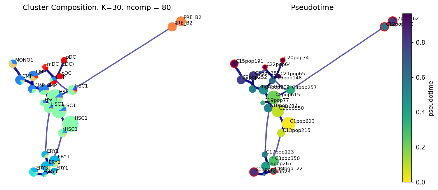
Cluster Level Trajectory Plots
fig, ax, ax1 = via.plot_piechart_viagraph(via_object=v0, show_legend=False)
fig.set_size_inches(12,5)
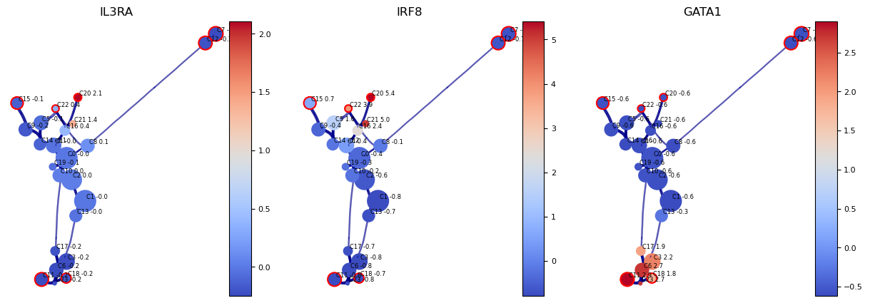
Visualise gene/feature graph
View the gene expression along the VIA graph. We use the computed HNSW small world graph in VIA to accelerate the gene imputation calculations (using similar approach to MAGIC) as follows:
df_ = pd.DataFrame(adata.X)
df_.columns = [i for i in adata.var_names]

gene_list_magic = ['IL3RA', 'IRF8', 'GATA1', 'GATA2', 'ITGA2B', 'MPO', 'CD79B', 'SPI1', 'CD34', 'CSF1R', 'ITGAX']

#optional to do gene expression imputation

df_magic = v0.do_impute(df_, magic_steps=3, gene_list=gene_list_magic)

fig, axs = via.plot_viagraph(via_object=v0, type_data='gene', df_genes=df_magic, gene_list=gene_list_magic[0:3], arrow_head=0.1)
fig.set_size_inches(15,5)
shape of transition matrix raised to power 3 (5780, 5780)
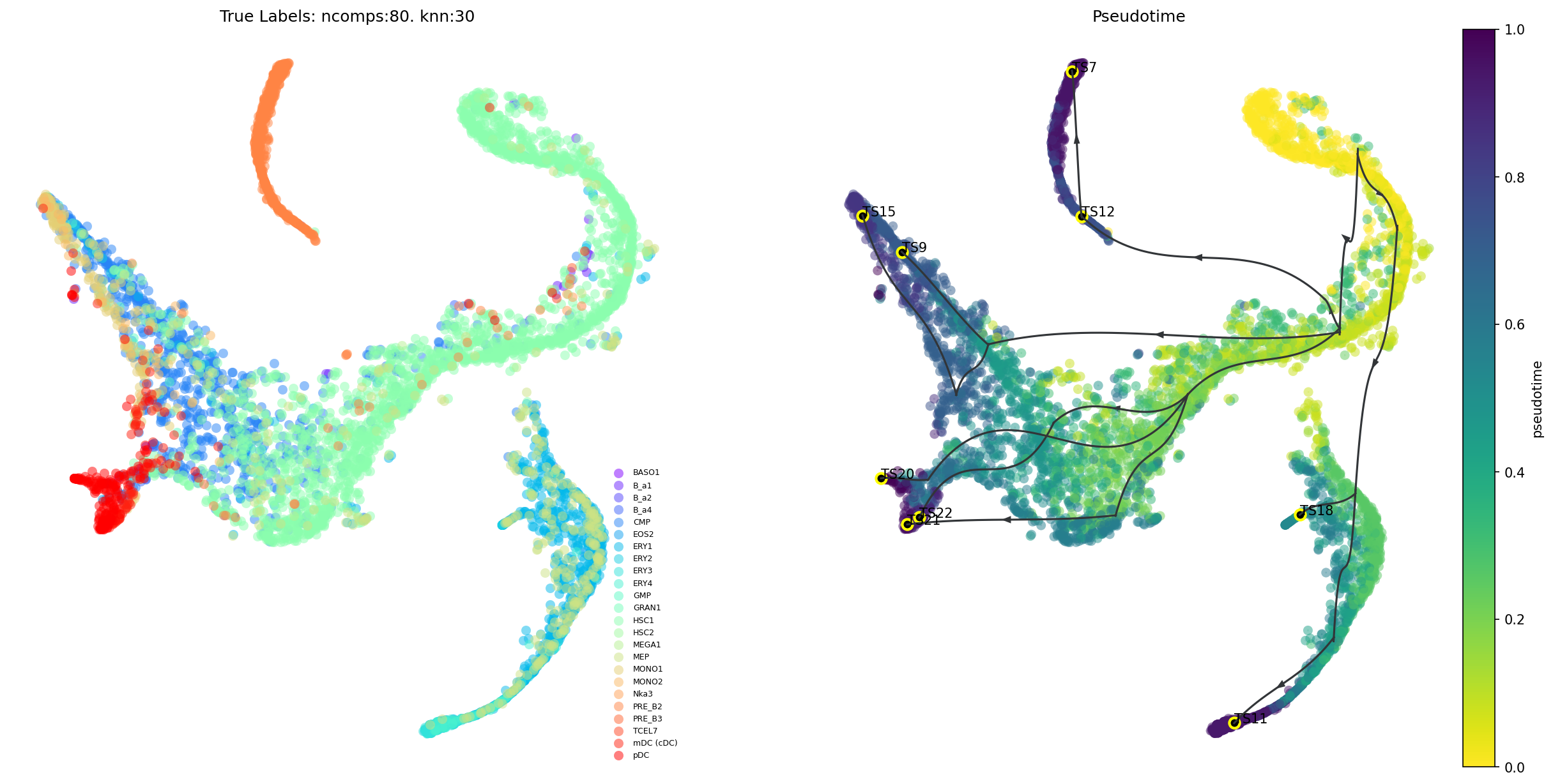
Trajectory projection
Visualize the overall VIA trajectory projected onto a 2D embedding (UMAP, Phate, TSNE etc) in different ways.
Draw the high-level clustergraph abstraction onto the embedding;
Draw high-edge resolution directed graph
Draw a vector field/stream plot of the more fine-grained directionality of cells along the trajectory projected onto an embedding.
Key Parameters:
scatter_size
scatter_alpha
linewidth
draw_all_curves (if too crowded, set to False)
fig, ax, ax1 = via.plot_trajectory_curves(via_object=v0,embedding=tsnem, draw_all_curves=False)
100% (11 of 11) |########################| Elapsed Time: 0:00:00 Time:  0:00:00
100% (11 of 11) |########################| Elapsed Time: 0:00:00 Time:  0:00:00
100% (11 of 11) |########################| Elapsed Time: 0:00:00 Time:  0:00:00
100% (11 of 11) |########################| Elapsed Time: 0:00:00 Time:  0:00:00
100% (11 of 11) |########################| Elapsed Time: 0:00:00 Time:  0:00:00
100% (11 of 11) |########################| Elapsed Time: 0:00:00 Time:  0:00:00
100% (11 of 11) |########################| Elapsed Time: 0:00:00 Time:  0:00:00
100% (11 of 11) |########################| Elapsed Time: 0:00:00 Time:  0:00:00
100% (11 of 11) |########################| Elapsed Time: 0:00:00 Time:  0:00:00
100% (11 of 11) |########################| Elapsed Time: 0:00:00 Time:  0:00:00
100% (11 of 11) |########################| Elapsed Time: 0:00:00 Time:  0:00:00
100% (11 of 11) |########################| Elapsed Time: 0:00:01 Time:  0:00:01
100% (11 of 11) |########################| Elapsed Time: 0:00:00 Time:  0:00:00
100% (11 of 11) |########################| Elapsed Time: 0:00:00 Time:  0:00:00
100% (11 of 11) |########################| Elapsed Time: 0:00:00 Time:  0:00:00
100% (11 of 11) |########################| Elapsed Time: 0:00:00 Time:  0:00:00
100% (11 of 11) |########################| Elapsed Time: 0:00:00 Time:  0:00:00
100% (11 of 11) |########################| Elapsed Time: 0:00:00 Time:  0:00:00
100% (11 of 11) |########################| Elapsed Time: 0:00:00 Time:  0:00:00
100% (11 of 11) |########################| Elapsed Time: 0:00:00 Time:  0:00:00
2023-10-30 13:55:26.039883	Super cluster 7 is a super terminal with sub_terminal cluster 7
2023-10-30 13:55:26.040203	Super cluster 9 is a super terminal with sub_terminal cluster 9
2023-10-30 13:55:26.040240	Super cluster 11 is a super terminal with sub_terminal cluster 11
2023-10-30 13:55:26.040271	Super cluster 12 is a super terminal with sub_terminal cluster 12
2023-10-30 13:55:26.040304	Super cluster 15 is a super terminal with sub_terminal cluster 15
2023-10-30 13:55:26.040351	Super cluster 18 is a super terminal with sub_terminal cluster 18
2023-10-30 13:55:26.040382	Super cluster 20 is a super terminal with sub_terminal cluster 20
2023-10-30 13:55:26.040412	Super cluster 21 is a super terminal with sub_terminal cluster 21
2023-10-30 13:55:26.040441	Super cluster 22 is a super terminal with sub_terminal cluster 22
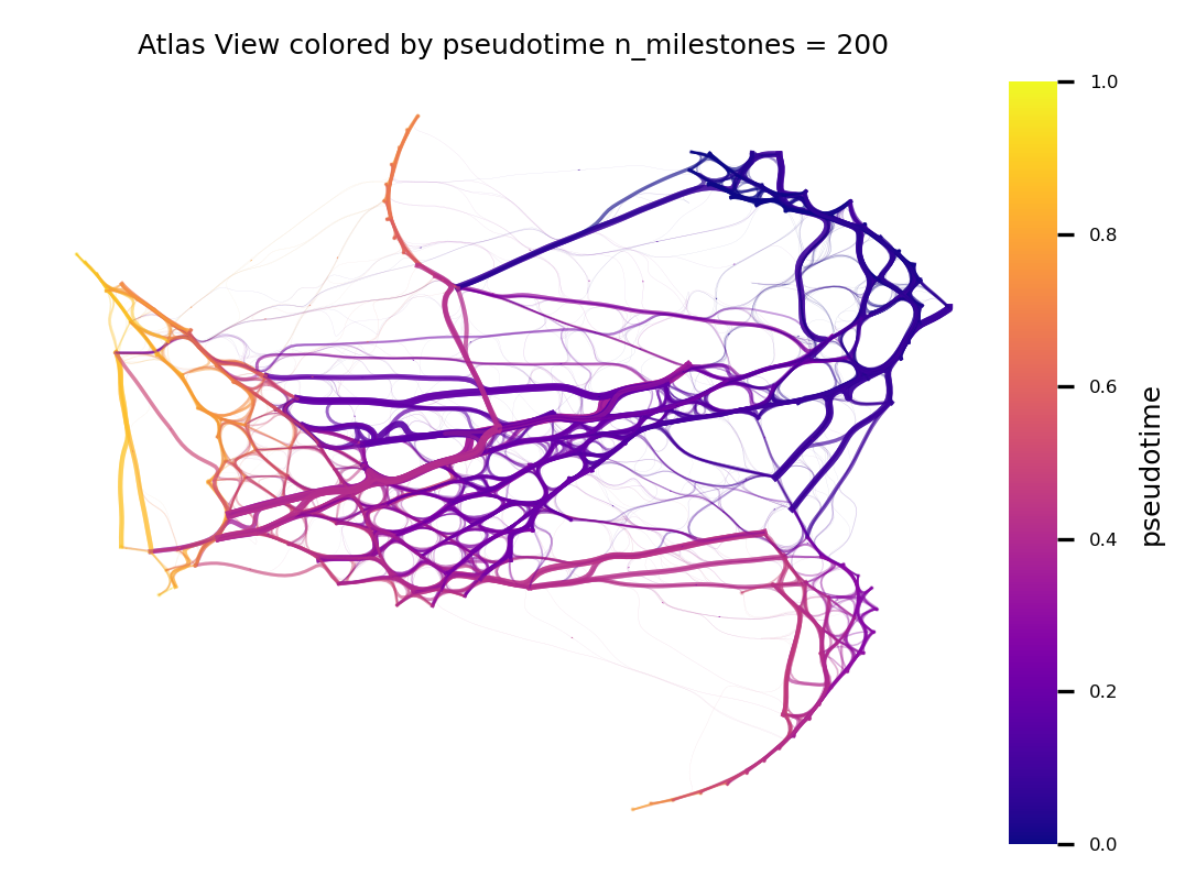
v0.embedding = tsnem
fig, ax = via.plot_atlas_view(via_object=v0,  n_milestones=150, sc_labels=adata.obs['label'], fontsize_labels=3, extra_title_text='Atlas View colored by pseudotime')
fig.set_size_inches(4,3)
inside add sc embedding second if
# edge plots can be made with different edge resolutions. Run hammerbundle_milestone_dict() to recompute the edges for plotting. Then provide the new hammerbundle as a parameter to plot_edge_bundle()
# it is better to compute the edges and save them to the via_object. this gives more control to the merging of edges
decay = 0.6 #increasing decay increasing merging of edges
i_bw = 0.02 #increasing bw increases merging of edges
global_visual_pruning = 0.5 #higher number retains more edges
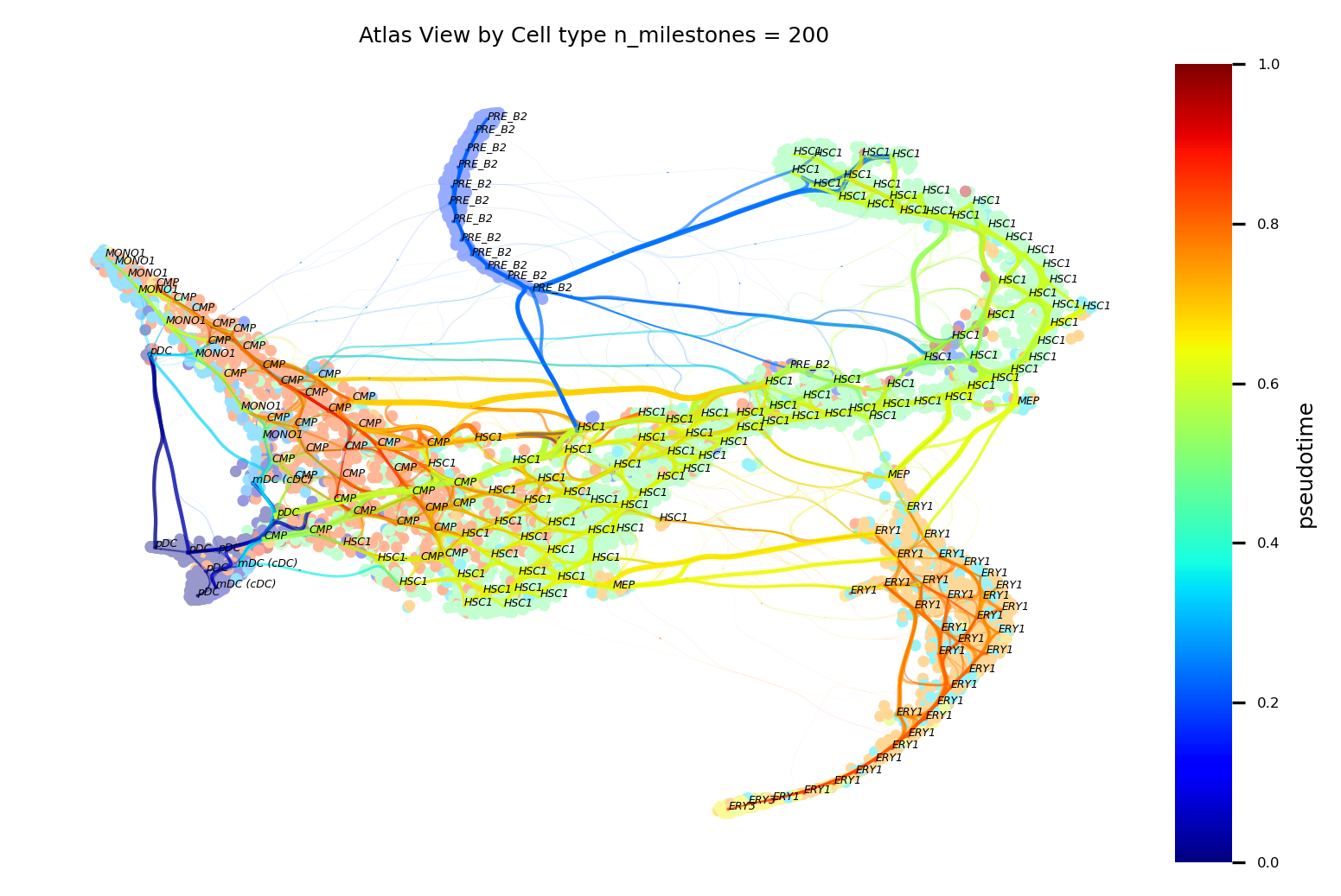
n_milestones = 200
v0.hammerbundle_milestone_dict= via.make_edgebundle_milestone(via_object=v0, n_milestones=n_milestones, decay=decay, initial_bandwidth=i_bw, global_visual_pruning=global_visual_pruning)
2023-10-30 15:03:28.888865	Start finding milestones
2023-10-30 15:03:33.107973	End milestones with 200
2023-10-30 15:03:33.130700	Recompute weights
2023-10-30 15:03:33.163942	pruning milestone graph based on recomputed weights
2023-10-30 15:03:33.165341	Graph has 1 connected components before pruning
2023-10-30 15:03:33.166303	Graph has 1 connected components after pruning
2023-10-30 15:03:33.166606	Graph has 1 connected components after reconnecting
2023-10-30 15:03:33.168703	regenerate igraph on pruned edges
2023-10-30 15:03:33.183040	Setting numeric label as single cell pseudotime for coloring edges
2023-10-30 15:03:33.235016	Making smooth edges
fig, ax = via.plot_atlas_view(via_object=v0,  add_sc_embedding=True, sc_labels_expression=adata.obs['label'], cmap='jet', sc_labels=adata.obs['label'], text_labels=True, extra_title_text='Atlas View by Cell type', fontsize_labels=3)
fig.set_size_inches(6,4)
inside add sc embedding second if
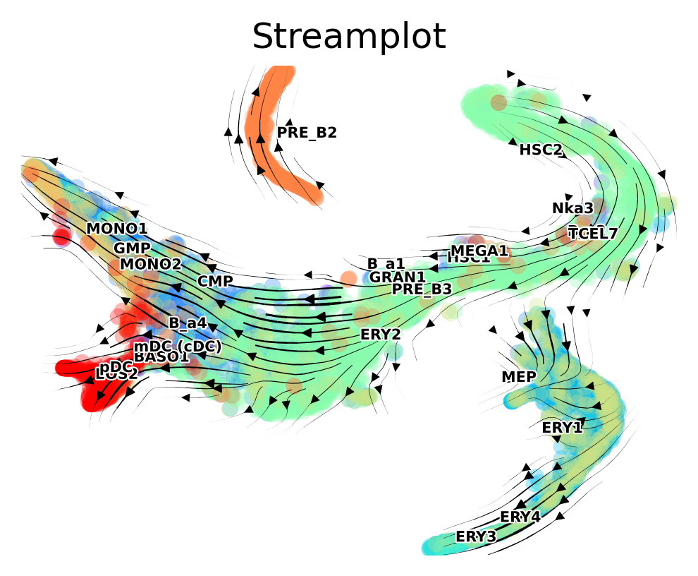
# via_streamplot() requires you to either provide an ndarray as embedding as an input parameter OR for via to have an embedding attribute
fig, ax = via.via_streamplot(v0, embedding=tsnem, density_grid=0.8, scatter_size=30, scatter_alpha=0.3, linewidth=0.5)
fig.set_size_inches(4,3)
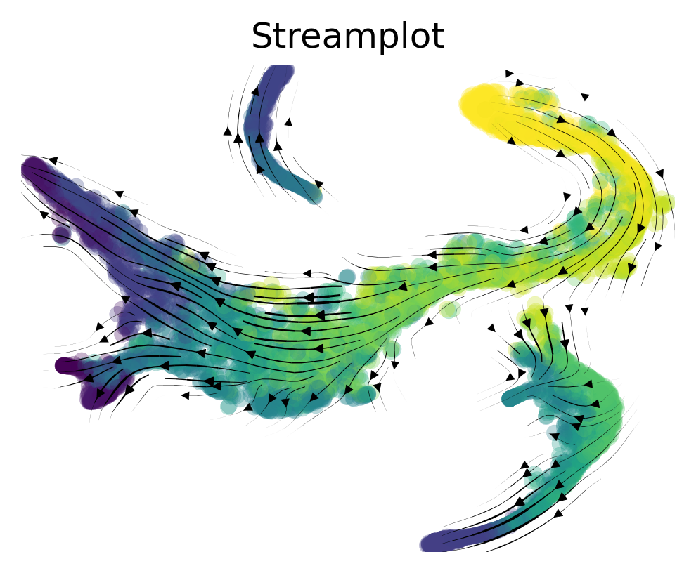
#Colored by pseudotime

fig, ax = via.via_streamplot(v0,density_grid=0.8, scatter_size=30, color_scheme='time', linewidth=0.5,
                             min_mass = 1, cutoff_perc = 5, scatter_alpha=0.3, marker_edgewidth=0.1,
                             density_stream = 2, smooth_transition=1, smooth_grid=0.5)
fig.set_size_inches(4,3)
Probabilistic pathways and Memory
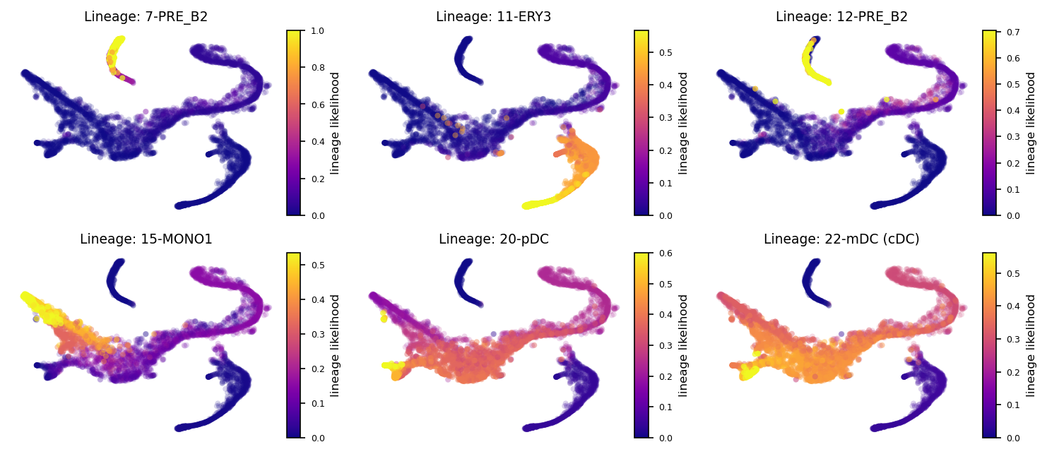
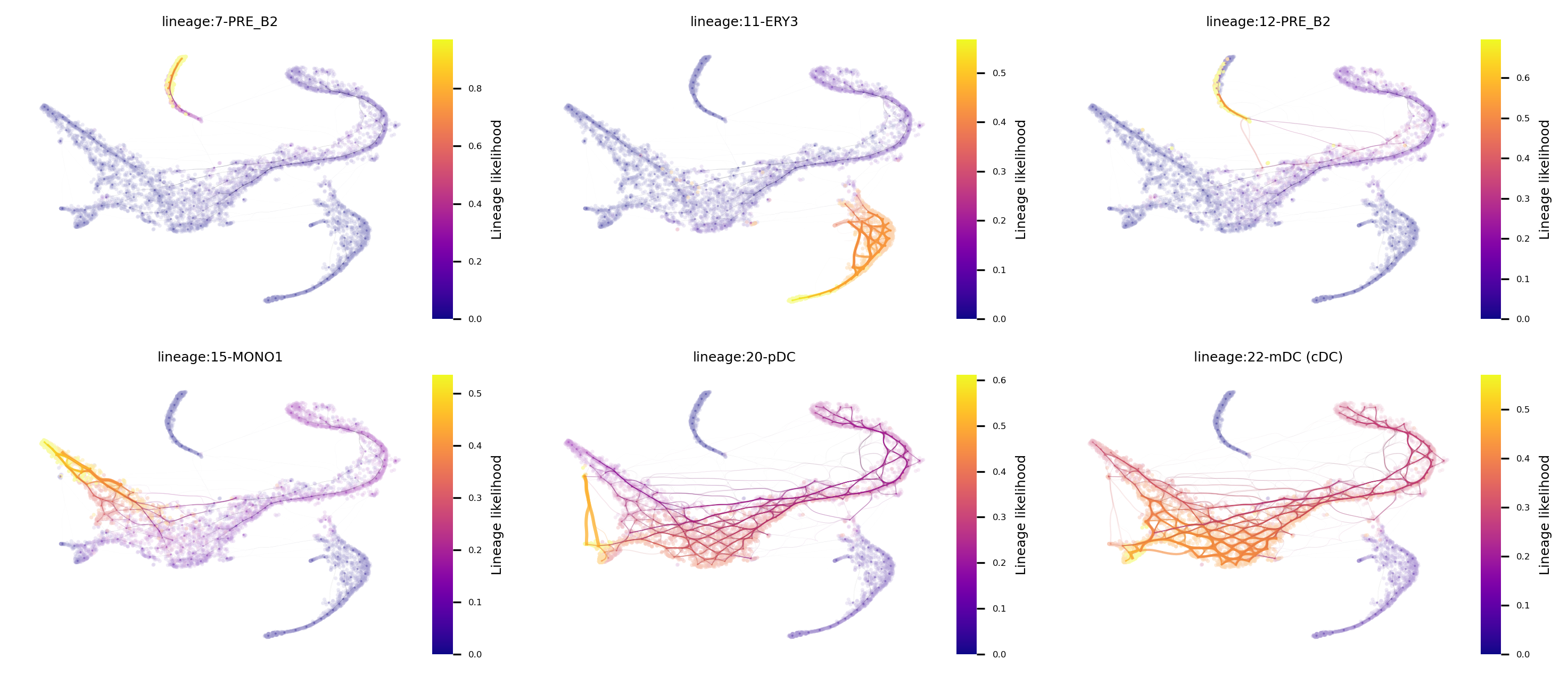
Visualize the probabilistic pathways from root to terminal state as indicated by the lineage likelihood. The higher the linage likelihood, the greater the potential of that particular cell to differentiate towards the terminal state of interest. Changing the memory paramater will alter the specificity of the lineage pathway. This can be visualized at the single-cell level but also combined with the Atlas View which visualizes cell-cell connectivity and pathways
Key Parameters:
marker_lineages (list) of terminal clusters
fig, axs= via.plot_sc_lineage_probability(via_object=v0, marker_lineages=[7,11,12,15,20,22], embedding=tsnem) #marker_lineages=v0.terminal_clusters to plot all
fig.set_size_inches(12,5)
2023-10-30 14:42:00.472388	Marker_lineages: [7, 11, 12, 15, 20, 22]
2023-10-30 14:42:00.476814	The number of components in the original full graph is 1
2023-10-30 14:42:00.476862	For downstream visualization purposes we are also constructing a low knn-graph
2023-10-30 14:42:05.171433	Check sc pb 0.9999999999999999
f getting majority comp
2023-10-30 14:42:05.475235	Cluster path on clustergraph starting from Root Cluster 1 to Terminal Cluster 7: [1, 2, 0, 4, 16, 8, 12, 7]
2023-10-30 14:42:05.475274	Cluster path on clustergraph starting from Root Cluster 1 to Terminal Cluster 11: [1, 13, 3, 6, 17, 11]
2023-10-30 14:42:05.475293	Cluster path on clustergraph starting from Root Cluster 1 to Terminal Cluster 12: [1, 2, 0, 4, 16, 8, 12]
2023-10-30 14:42:05.475311	Cluster path on clustergraph starting from Root Cluster 1 to Terminal Cluster 15: [1, 2, 0, 4, 16, 5, 15]
2023-10-30 14:42:05.475328	Cluster path on clustergraph starting from Root Cluster 1 to Terminal Cluster 18: [1, 13, 3, 18]
2023-10-30 14:42:05.475345	Cluster path on clustergraph starting from Root Cluster 1 to Terminal Cluster 20: [1, 2, 0, 4, 16, 20]
2023-10-30 14:42:05.475362	Cluster path on clustergraph starting from Root Cluster 1 to Terminal Cluster 22: [1, 2, 0, 4, 22]
2023-10-30 14:42:05.605789	Revised Cluster level path on sc-knnGraph from Root Cluster 1 to Terminal Cluster 7 along path: [1, 1, 1, 8, 12, 12, 12]
2023-10-30 14:42:05.640568	Revised Cluster level path on sc-knnGraph from Root Cluster 1 to Terminal Cluster 11 along path: [1, 1, 2, 6, 11, 11, 11, 11]
2023-10-30 14:42:05.678481	Revised Cluster level path on sc-knnGraph from Root Cluster 1 to Terminal Cluster 12 along path: [1, 1, 1, 8, 12, 12, 12, 12]
2023-10-30 14:42:05.724775	Revised Cluster level path on sc-knnGraph from Root Cluster 1 to Terminal Cluster 15 along path: [1, 1, 2, 9, 15]
2023-10-30 14:42:05.761232	Revised Cluster level path on sc-knnGraph from Root Cluster 1 to Terminal Cluster 20 along path: [1, 1, 1, 8, 20, 20, 20, 20]
2023-10-30 14:42:05.805373	Revised Cluster level path on sc-knnGraph from Root Cluster 1 to Terminal Cluster 22 along path: [1, 1, 1, 8, 22, 22, 22]
fig, axs= via.plot_atlas_view(via_object=v0, lineage_pathway=[7,11,12,15,20,22]) #marker_lineages=v0.terminal_clusters to plot all
fig.set_size_inches(12,5)
location of 7 is at [0] and 0
location of 11 is at [1] and 1
location of 12 is at [2] and 2
location of 15 is at [3] and 3
location of 20 is at [5] and 5
location of 22 is at [6] and 6
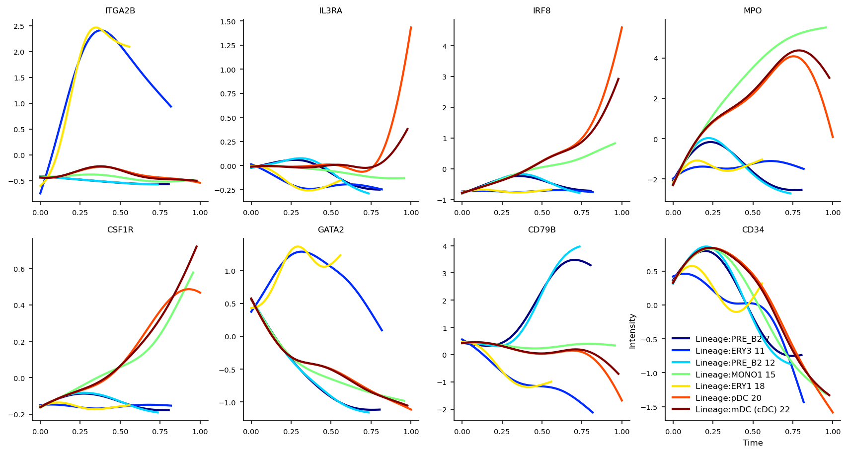
Gene Dynamics
The gene dynamics along pseudotime for all detected lineages are automatically inferred by VIA. These can be interpreted as the change in gene expression along any given lineage.
Key Parameters
n_splines
spline_order
gene_exp (dataframe) single-cell level gene expression of select genes (gene imputation is an optional pre-step)
marker_genes =['ITGA2B', 'IL3RA', 'IRF8', 'MPO', 'CSF1R', 'GATA2', 'CD79B', 'CD34']
df = pd.DataFrame(adata.X, columns = adata.var_names)
df_magic = v0.do_impute(df, magic_steps=3, gene_list=gene_list_magic) #optional
fig, axs=via.get_gene_expression(via_object=v0, gene_exp=df_magic[marker_genes])
fig.set_size_inches(14,7)
shape of transition matrix raised to power 3 (5780, 5780)
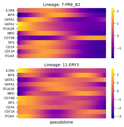
Gene Dynamics
Heatmaps of genes along pseudotimetime
Key Parameters
df_gene_exp (dataframe) single-cell level gene expression of selected genes
marker_lineages (list, optional) to specify which lineages to plot heatmaps for
fig, axs = via.plot_gene_trend_heatmaps(via_object=v0, df_gene_exp=df_magic, cmap='plasma',
                             marker_lineages=[7,11])
fig.set_size_inches(5,5)
branches [7, 11]
Various Visualizations
Visualizations of the trajectory can be plotted at various edge resolutions
Edge bundle plot
Key Parameters (default):
alpha_bundle_factor=1
linewidth_bundle=2
cmap:str = ‘plasma_r’
size_scatter:int=2
alpha_scatter:float = 0.2
headwidth_bundle=0.1
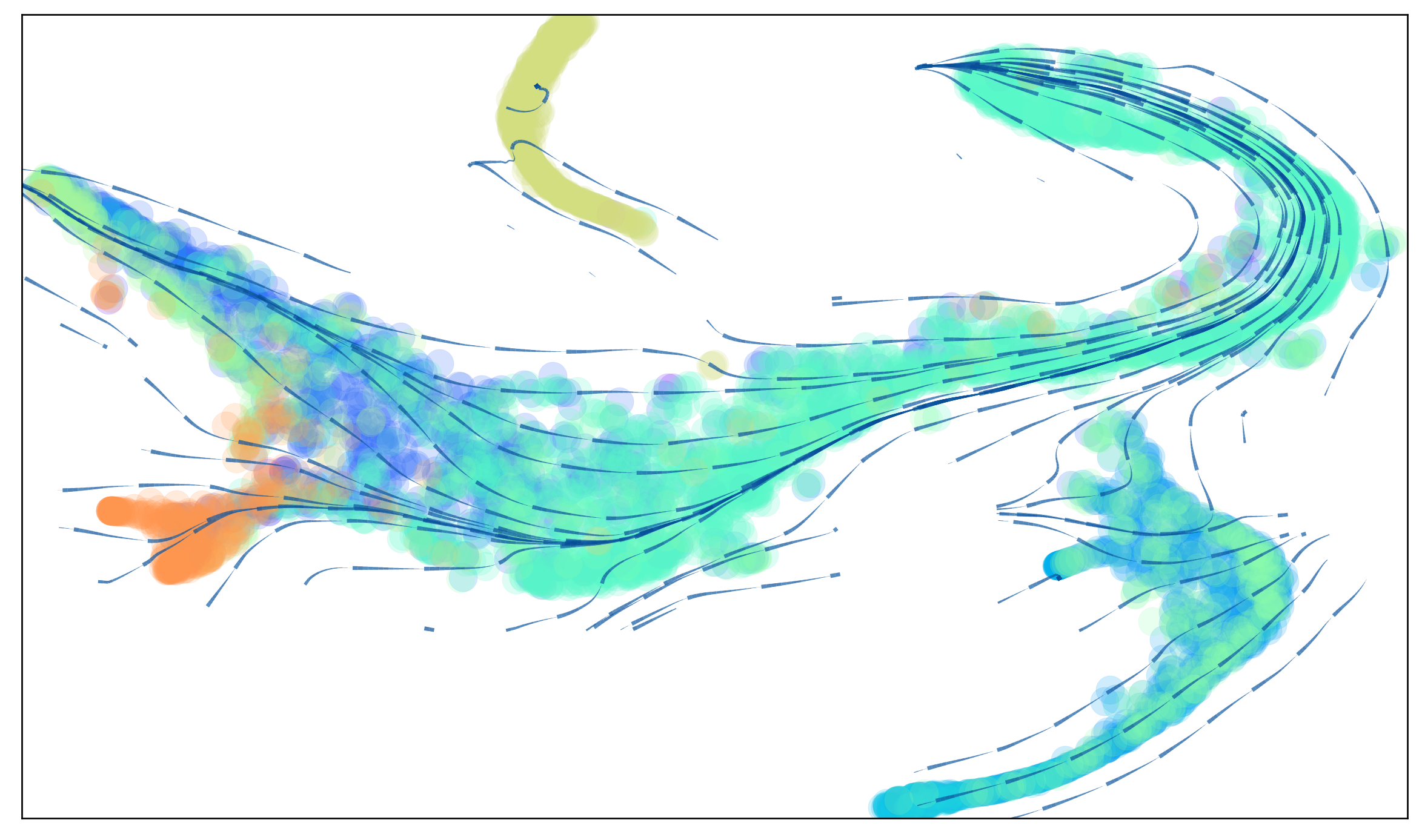
Animated Stream plot
sc.settings.set_figure_params(dpi=120, facecolor='white')
#the streamlines load very slowly through the Notebook, so see the code below to open the file and view the animation properly
via.animated_streamplot(v0, embedding=tsnem, cmap_stream='Blues', scatter_size=200, scatter_alpha=0.2, marker_edgewidth=0.15,
                        density_grid=0.7, linewidth=0.1, segment_length=1.5, saveto='/home/shobi/Trajectory/Datasets/HumanCD34/HumanCD34_animation_Jan3.gif')
2023-01-03 09:32:23.524989 Inside animated. File will be saved to location /home/shobi/Trajectory/Datasets/HumanCD34/HumanCD34_animation_Jan3.gif
0%| | 0/250 [00:00<?, ?it/s]
total number of stream lines 201
(<Figure size 1200x720 with 1 Axes>, <AxesSubplot:>)
from IPython.display import Image

with open('./Figures/HumanCD34_animation.gif','rb') as file:
    display(Image(file.read()))
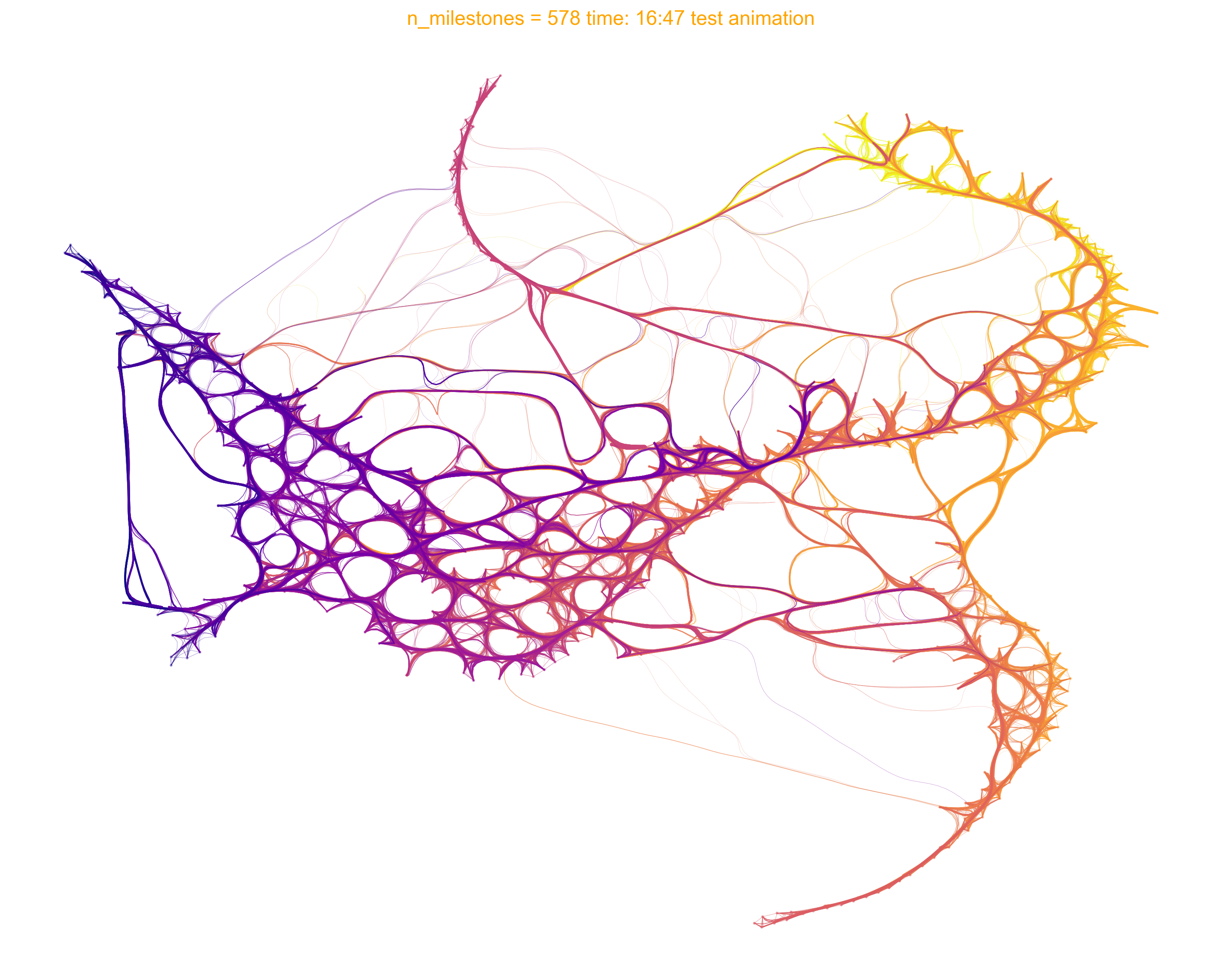
Animated edge bundle plot
via.animate_edge_bundle(via_object=v0, extra_title_text='test animation', n_milestones=None,
                        saveto='./Figures/human_edgebundle_test.gif')
making hammerbundle
2022-11-08 16:46:46.082215	Start kmeans milestone
2022-11-08 16:46:50.162267	End kmeans milestone
2022-11-08 16:46:50.230431	Recompute weights
2022-11-08 16:46:50.348908	pruning milestone graph based on recomputed weights
2022-11-08 16:46:50.358479	Graph has 1 connected components before pruning
2022-11-08 16:46:50.358479	Graph has 1 connected components before pruning
2022-11-08 16:46:50.368028	regenerate igraph on pruned edges
2022-11-08 16:46:50.456737	make node dataframe
2022-11-08 16:46:50.472879	Setting numeric label as time_series_labels or other sequential metadata for coloring edges
2022-11-08 16:46:50.592365	Hammer bundling
seg weight 0.1311759587041706
MovieWriter imagemagick unavailable; using Pillow instead.
2022-11-08 16:47:46.937861	Finished plotting edge bundle
times series order set [0, 1, 2, 3, 4, 5, 6, 7, 8, 9, 10]
number cycles if no time_series labels given 40.0
complete animate
inside update 0 out of 120
inside update 0 out of 120
inside update 1 out of 120
inside update 2 out of 120
inside update 3 out of 120
inside update 4 out of 120
inside update 5 out of 120
inside update 6 out of 120
inside update 7 out of 120
inside update 8 out of 120
inside update 9 out of 120
inside update 10 out of 120
inside update 11 out of 120
inside update 12 out of 120
inside update 13 out of 120
inside update 14 out of 120
inside update 15 out of 120
inside update 16 out of 120
inside update 17 out of 120
inside update 18 out of 120
inside update 19 out of 120
inside update 20 out of 120
inside update 21 out of 120
inside update 22 out of 120
inside update 23 out of 120
inside update 24 out of 120
inside update 25 out of 120
inside update 26 out of 120
inside update 27 out of 120
inside update 28 out of 120
inside update 29 out of 120
inside update 30 out of 120
inside update 31 out of 120
inside update 32 out of 120
inside update 33 out of 120
inside update 34 out of 120
inside update 35 out of 120
inside update 36 out of 120
inside update 37 out of 120
inside update 38 out of 120
inside update 39 out of 120
inside update 40 out of 120
inside update 41 out of 120
inside update 42 out of 120
inside update 43 out of 120
inside update 44 out of 120
inside update 45 out of 120
inside update 46 out of 120
inside update 47 out of 120
inside update 48 out of 120
inside update 49 out of 120
inside update 50 out of 120
inside update 51 out of 120
inside update 52 out of 120
inside update 53 out of 120
inside update 54 out of 120
inside update 55 out of 120
inside update 56 out of 120
inside update 57 out of 120
inside update 58 out of 120
inside update 59 out of 120
inside update 60 out of 120
inside update 61 out of 120
inside update 62 out of 120
inside update 63 out of 120
inside update 64 out of 120
inside update 65 out of 120
inside update 66 out of 120
inside update 67 out of 120
inside update 68 out of 120
inside update 69 out of 120
inside update 70 out of 120
inside update 71 out of 120
inside update 72 out of 120
inside update 73 out of 120
inside update 74 out of 120
inside update 75 out of 120
inside update 76 out of 120
inside update 77 out of 120
inside update 78 out of 120
inside update 79 out of 120
inside update 80 out of 120
inside update 81 out of 120
inside update 82 out of 120
inside update 83 out of 120
inside update 84 out of 120
inside update 85 out of 120
inside update 86 out of 120
inside update 87 out of 120
inside update 88 out of 120
inside update 89 out of 120
inside update 90 out of 120
inside update 91 out of 120
inside update 92 out of 120
inside update 93 out of 120
inside update 94 out of 120
inside update 95 out of 120
inside update 96 out of 120
inside update 97 out of 120
inside update 98 out of 120
inside update 99 out of 120
inside update 100 out of 120
inside update 101 out of 120
inside update 102 out of 120
inside update 103 out of 120
inside update 104 out of 120
inside update 105 out of 120
inside update 106 out of 120
inside update 107 out of 120
inside update 108 out of 120
inside update 109 out of 120
inside update 110 out of 120
inside update 111 out of 120
inside update 112 out of 120
inside update 113 out of 120
inside update 114 out of 120
inside update 115 out of 120
inside update 116 out of 120
inside update 117 out of 120
inside update 118 out of 120
inside update 119 out of 120
saved animation
from IPython.display import Image
with open('/home/user/Github_local/VIA/Figures/human_edgebundle_test.gif','rb') as file:
    display(Image(file.read()))