3. Via 2.0 Cartography on Zebrahub (Visualization)
This tutorial focuses on how to generate the Via2.0 Zebrahub Atlas View. The TI analysis is shown in Tutorial #2
import scanpy as sc
import matplotlib.pyplot as plt
import pandas as pd
import numpy as np
import pyVIA.core as via
from datetime import datetime
Load the data
Data has been filtered and library normalized. Data is annotated with time/stage, cluster labels, and cell type labels (coarse and fine)
print(f'{datetime.now()}\tStart reading data')
adata=sc.read_h5ad( filename='/home/user/Trajectory/Datasets/Zebrafish_Lange2023/Rawdata/Zebrahub_data_via.h5ad')
#compute PCA
adata.uns['log1p']['base'] = None #fix for small bug in scanpy #see https://github.com/theislab/single-cell-tutorial/issues/97
sc.pp.highly_variable_genes(adata, n_top_genes=2000)
sc.tl.pca(adata, n_comps=100)
print(adata)
2024-02-06 16:48:28.584723	Start reading data
AnnData object with n_obs × n_vars = 119457 × 28187
    obs: 'n_genes', 'n_counts', 'fish', 'timepoint_cluster', 'n_genes_by_counts', 'total_counts', 'total_counts_mt', 'pct_counts_mt', 'total_counts_nc', 'pct_counts_nc', 'developmental_stage', 'timepoint', 'zebrafish_anatomy_ontology_class', 'zebrafish_anatomy_ontology_id', 'parc', 'kmeans50', 'celltype_extrainfo', 'zebrafish_anatomy_ontology_class_shobi', 'adjusted_timepoint', 'bool_list', 'global annotation', 'time_coarse_cell_type', 'time_fine_cell_type', 'parc_cluster', 'parc_cluster_and_cell_type'
    var: 'gene_ids', 'feature_types', 'genome', 'mt', 'nc', 'n_cells_by_counts', 'mean_counts', 'pct_dropout_by_counts', 'total_counts', 'n_cells', 'highly_variable', 'means', 'dispersions', 'dispersions_norm'
    uns: 'global_annotation_colors', 'hvg', 'log1p', 'pca', 'timepoint_colors', 'zebrafish_anatomy_ontology_class_colors', 'zebrafish_anatomy_ontology_id_colors'
    obsm: 'X_U', 'X_Via2_Atlas', 'X_pca', 'X_umap'
    varm: 'PCs'
    layers: 'counts'
Extract some annotations
n_cells = adata.shape[0]
print('cells is', n_cells)
parc_cluster = [i for i in adata.obs['parc_cluster']]
parc_cluster_and_cell_type = [i for i in adata.obs['parc_cluster_and_cell_type']]
coarse_cell_type = [i for i in adata.obs['zebrafish_anatomy_ontology_class']]
fine_cell_type = [i for i in adata.obs['zebrafish_anatomy_ontology_class_shobi']] #consolidated annotaions from individual time point files
coarse_fine_cell_type = [coarse_cell_type[i] + fine_cell_type[i] for i in range(n_cells)]
time_point_numeric = [i for i in adata.obs['adjusted_timepoint']] #assigned a numeric value to each stage (e.g. 5hpf is 5, 10hpf is 10,...)
early_cell_type = [i if str(i) != 'nan' else '' for i in adata.obs['global annotation']]

hybrid_cell_time = [str(fine_cell_type[i]) + '_'+early_cell_type[i]+'_'+str(time_point_numeric[i]) for i in range(n_cells)] #labels of early stage cells which was provided for cells <24hpf also included
parc_numeric_cluster_labels = [i for i in adata.obs['parc']]
parc_cluster = [i for i in adata.obs['parc_cluster']]
cells is 119457
Find a suitable root
root_str = 'paraxial mesoderm_Somites_0'
loc_root = np.where(np.asarray(hybrid_cell_time) == root_str)[0] #'paraxial mesoderm_PSM_0' 1 cell , 'paraxial mesoderm_Somites_0' has 51 cells, 'paraxial mesoderm_Muscle_0', 'tail bud_NMPs_0'
root = [loc_root[0]]
n_pcs = 100
print(f'{datetime.now()}\troot is cell number  {root[0]} of type {fine_cell_type[root[0]]}')
2024-02-06 16:49:16.395417 root is cell number 2604 of type paraxial mesoderm
Initialize parameters
knn=30
time_series = True  # True
memory = 10
jac_std_global = 1  # 1 is used in all the umap csv files
random_seed = 0#1  # 0
knn_sequential = 15  # 5 forviagraphs #15 for embedding
t_diff_step = 2
do_gaussian_kernel_edgeweights = False
edgebundle_pruning_twice = True
edgepruning_clustering_resolution = 0.15  # 0.15 viagraph and embedding
edgebundle_pruning = 0.05  # 0.15
neighboring_terminal_states_threshold = 4  # 3
viagraph_decay = 0.6  # 0.7, 0.9
max_vis_out = 2
Set terminal states (optional)
# The parameter "user_defined_terminal_group" is being set to a list of group level annotations corresponding to the provided true_label. These were terminal fates detected in previous runs and saved for reproducability.
# This parameter can also be left to its default user_defined_terminal_group = []. the results should be similar.
user_defined_cellfates= ['0_cartilage element', '2_dermis', '49_fin',
                                          '67_pharyngeal arch', '120_cranial cartilage',
                                          '1_forebrain', '71_neuron', '89_diencephalon',
                                          '136_radial glial cell',
                                          '10_epidermal cell', '83_neuromast',
                                          '145_enteric musculature', '55_myotome',
                                          '46_hematopoietic cell',                                          '102_vasculature', '127_Muller cell', '105_oligodendrocyte',                            '69_liver', '90_pharynx',
                                          '95_intestine']
Initialize and Run the Via2.0 Class
# Initialize and Run the Via2.0 Class
print(f'{datetime.now()}\tRun Via2.0')

v0 = via.VIA(adata.obsm['X_pca'][:, 0:n_pcs], true_label=parc_cluster_and_cell_type,
             labels=parc_cluster, knn=knn, memory=memory,
             user_defined_terminal_group=user_defined_cellfates,
             edgepruning_clustering_resolution=edgepruning_clustering_resolution,
             neighboring_terminal_states_threshold=neighboring_terminal_states_threshold,
             too_big_factor=0.3, resolution_parameter=1,
             root_user=root, dataset='', random_seed=random_seed,
             is_coarse=True, preserve_disconnected=False, pseudotime_threshold_TS=40, x_lazy=0.99,
             do_gaussian_kernel_edgeweights=do_gaussian_kernel_edgeweights,
             alpha_teleport=0.99, edgebundle_pruning=edgebundle_pruning, edgebundle_pruning_twice=True,
             time_series=time_series, time_series_labels=time_point_numeric, knn_sequential=knn_sequential,
             knn_sequential_reverse=knn_sequential, t_diff_step=t_diff_step,
             do_compute_embedding=False)

v0.run_VIA()
2024-02-06 16:49:16.446582	Run Via2.0
2024-02-06 16:49:16.453681	Running VIA over input data of 119457 (samples) x 100 (features)
2024-02-06 16:49:16.453681	Knngraph has 30 neighbors
2024-02-06 16:49:49.943120	Using time series information to guide knn graph construction
2024-02-06 16:49:49.954230	Time series ordered set [0, 5, 10, 15, 20, 25, 30, 35, 40, 45]
2024-02-06 16:50:36.547252	Shape neighbors (119457, 30) and sequential neighbors (119457, 30)
2024-02-06 16:50:36.600487	Shape augmented neighbors (119457, 60)
2024-02-06 16:50:36.651840	Actual average allowable time difference between nodes is 10.0
2024-02-06 16:50:55.131081	Finished global pruning of 30-knn graph used for clustering at level of 0.15. Kept 46.9 % of edges.
2024-02-06 16:50:55.445815	Number of connected components used for clustergraph  is 1
2024-02-06 16:51:17.750064	Using predfined labels provided by user (this must be provided as an array)
2024-02-06 16:51:17.750064	Making cluster graph. Global cluster graph pruning level: 0.15
2024-02-06 16:51:19.093352	Graph has 1 connected components before pruning
2024-02-06 16:51:19.108996	Graph has 1 connected components after pruning
2024-02-06 16:51:19.108996	Graph has 1 connected components after reconnecting
2024-02-06 16:51:19.108996	48.0% links trimmed from local pruning relative to start
2024-02-06 16:51:19.108996	88.8% links trimmed from global pruning relative to start
2024-02-06 16:51:19.108996	Graph has 1 connected components before pruning
2024-02-06 16:51:19.108996	Graph has 3 connected components after pruning
2024-02-06 16:51:19.124624	Graph has 1 connected components after reconnecting
2024-02-06 16:51:19.124624	48.0% links trimmed from local pruning relative to start
2024-02-06 16:51:19.124624	92.1% links trimmed from global pruning relative to start
2024-02-06 16:51:19.124624	component number 0 out of  [0]
C:\Users\Kevin tsia\anaconda3\envs\via2\lib\site-packages\scipy\sparse\_index.py:103: SparseEfficiencyWarning: Changing the sparsity structure of a csr_matrix is expensive. lil_matrix is more efficient.
  self._set_intXint(row, col, x.flat[0])
2024-02-06 16:51:20.255203	The root index, 2604 provided by the user belongs to cluster number 97 and corresponds to cell type 97_paraxial mesoderm
2024-02-06 16:51:20.404829	Computing lazy-teleporting expected hitting times
2024-02-06 16:51:31.983877	 ended all multiprocesses, will retrieve and reshape
try rw2 hitting times setup
start computing walks with rw2 method
g.indptr.size, 147
C:\Users\Kevin tsia\anaconda3\envs\via2\lib\site-packages\pecanpy\graph.py:90: UserWarning: WARNING: Implicitly set node IDs to the canonical node ordering due to missing IDs field in the raw CSR npz file. This warning message can be suppressed by setting implicit_ids to True in the read_npz function call, or by setting the --implicit_ids flag in the CLI
  warnings.warn(
memory for rw2 hittings times  2. Using rw2 based pt
do scaling of pt
2024-02-06 16:51:41.963854	Terminal cluster list based on user defined cells/groups: [('0_cartilage element', 0), ('2_dermis', 2), ('49_fin', 49), ('67_pharyngeal arch', 67), ('120_cranial cartilage', 120), ('1_forebrain', 1), ('71_neuron', 71), ('89_diencephalon', 89), ('136_radial glial cell', 136), ('10_epidermal cell', 10), ('83_neuromast', 83), ('145_enteric musculature', 145), ('55_myotome', 55), ('46_hematopoietic cell', 46), ('102_vasculature', 102), ('127_Muller cell', 127), ('105_oligodendrocyte', 105), ('69_liver', 69), ('90_pharynx', 90), ('95_intestine', 95)]
2024-02-06 16:51:41.963854	Terminal clusters corresponding to unique lineages in this component are [0, 2, 49, 67, 120, 1, 71, 89, 136, 10, 83, 145, 55, 46, 102, 127, 105, 69, 90, 95]
TESTING rw2_lineage probability at memory 10
testing rw2 lineage probability at memory 10
g.indptr.size, 147
C:\Users\Kevin tsia\anaconda3\envs\via2\lib\site-packages\pecanpy\graph.py:90: UserWarning: WARNING: Implicitly set node IDs to the canonical node ordering due to missing IDs field in the raw CSR npz file. This warning message can be suppressed by setting implicit_ids to True in the read_npz function call, or by setting the --implicit_ids flag in the CLI
  warnings.warn(
2024-02-06 16:51:48.486988	 Cluster or terminal cell fate 0 is reached 265.0 times
2024-02-06 16:51:48.683785	 Cluster or terminal cell fate 2 is reached 321.0 times
2024-02-06 16:51:48.923914	 Cluster or terminal cell fate 49 is reached 38.0 times
2024-02-06 16:51:49.118724	 Cluster or terminal cell fate 67 is reached 326.0 times
2024-02-06 16:51:49.340747	 Cluster or terminal cell fate 120 is reached 169.0 times
2024-02-06 16:51:49.568767	 Cluster or terminal cell fate 1 is reached 65.0 times
2024-02-06 16:51:49.816750	 Cluster or terminal cell fate 71 is reached 45.0 times
2024-02-06 16:51:50.007561	 Cluster or terminal cell fate 89 is reached 417.0 times
2024-02-06 16:51:50.233503	 Cluster or terminal cell fate 136 is reached 116.0 times
2024-02-06 16:51:50.461331	 Cluster or terminal cell fate 10 is reached 71.0 times
2024-02-06 16:51:50.692439	 Cluster or terminal cell fate 83 is reached 30.0 times
2024-02-06 16:51:50.925563	 Cluster or terminal cell fate 145 is reached 116.0 times
2024-02-06 16:51:51.169573	 Cluster or terminal cell fate 55 is reached 45.0 times
2024-02-06 16:51:51.405499	 Cluster or terminal cell fate 46 is reached 25.0 times
2024-02-06 16:51:51.625457	 Cluster or terminal cell fate 102 is reached 124.0 times
2024-02-06 16:51:51.854602	 Cluster or terminal cell fate 127 is reached 109.0 times
2024-02-06 16:51:52.087725	 Cluster or terminal cell fate 105 is reached 59.0 times
2024-02-06 16:51:52.314733	 Cluster or terminal cell fate 69 is reached 47.0 times
2024-02-06 16:51:52.546824	 Cluster or terminal cell fate 90 is reached 66.0 times
2024-02-06 16:51:52.788913	 Cluster or terminal cell fate 95 is reached 40.0 times
2024-02-06 16:51:53.453693	There are (20) terminal clusters corresponding to unique lineages {0: '0_pectoral fin', 2: '2_dermis', 49: '49_fin', 67: '67_pharyngeal arch', 120: '120_cranial cartilage', 1: '1_forebrain', 71: '71_neuron', 89: '89_diencephalon', 136: '136_radial glial cell', 10: '10_epidermal cell', 83: '83_neuromast', 145: '145_enteric musculature', 55: '55_myotome', 46: '46_hematopoietic cell', 102: '102_vasculature', 127: '127_Muller cell', 105: '105_oligodendrocyte', 69: '69_liver', 90: '90_pharynx', 95: '95_intestine'}
2024-02-06 16:51:53.453693	Begin projection of pseudotime and lineage likelihood
2024-02-06 16:52:02.358324	Start reading data
2024-02-06 16:52:02.358324	Correlation of Via pseudotime with developmental stage 73.33 %
2024-02-06 16:52:02.400584	Cluster graph layout based on forward biasing
2024-02-06 16:52:02.426671	Graph has 1 connected components before pruning
2024-02-06 16:52:02.432658	Graph has 58 connected components after pruning
2024-02-06 16:52:02.478882	Graph has 1 connected components after reconnecting
2024-02-06 16:52:02.479882	67.2% links trimmed from local pruning relative to start
2024-02-06 16:52:02.479882	80.4% links trimmed from global pruning relative to start
2024-02-06 16:52:02.479882	Additional Visual cluster graph pruning for edge bundling at level: 0.15
2024-02-06 16:52:02.481883	Make via clustergraph edgebundle
C:\Users\Kevin tsia\anaconda3\envs\via2\lib\site-packages\scipy\sparse\_index.py:103: SparseEfficiencyWarning: Changing the sparsity structure of a csr_matrix is expensive. lil_matrix is more efficient.
  self._set_intXint(row, col, x.flat[0])
2024-02-06 16:52:05.635522	Hammer dims: Nodes shape: (146, 2) Edges shape: (890, 3)
2024-02-06 16:52:05.853588	Time elapsed 143.6 seconds
Computing the Atlas View
Set parameter init_pos
‘via’ : uses via graph to initialize embedding
‘spectral’ : uses normalized Laplacian of the fuzzy 1-skeleton
n_cell x 2 dimensional array preset by the user
Once you have the single cell atlas embedding, you can compute the edge layout and generate the full Atlas View
compute_atlas_embedding = True
if compute_atlas_embedding:
    # STEP 3
    print(f'{datetime.now()}\tStart Atlas embedding computation')
    atlas_embedding = via.via_atlas_emb(via_object=v0, init_pos='via', min_dist=0.2)
else: atlas_embedding = embedding=adata.obsm['X_Via2_Atlas'] #use pre-saved embedding

v0.embedding = atlas_embedding #remember to pass this onto the via_object
2024-02-06 16:52:05.878707	Start Atlas embedding computation
X-input (119457, 100)
len membership and n_cells 119457 119457
n cell 119457
2024-02-06 16:52:05.878707	Computing embedding on sc-Viagraph
2024-02-06 16:52:10.671518	using via cluster graph to initialize embedding
(119457, 100)
	completed  0  /  100 epochs
	completed  10  /  100 epochs
	completed  20  /  100 epochs
	completed  30  /  100 epochs
	completed  40  /  100 epochs
	completed  50  /  100 epochs
	completed  60  /  100 epochs
	completed  70  /  100 epochs
	completed  80  /  100 epochs
	completed  90  /  100 epochs
Re-orient (optional)
If you want to apply a rotation transformation on the embedding
#re-orient/rotate. This can be skipped. Only use it if neceseary First plot out the atlas_embedding (code in next snipped) and see if you want to rotate it so the early cells are on the LHS. import math theta_deg = 180 theta_radians = math.sin(math.radians(theta_deg)) R = np.array([[math.cos(theta_radians), -math.sin(theta_radians)],[math.sin(theta_radians),math.cos(theta_radians)]]) atlas_embedding_ = np.matmul(R,atlas_embedding.T) atlas_embedding_=atlas_embedding.T v0.embedding = atlas_embedding_
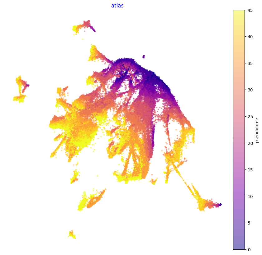
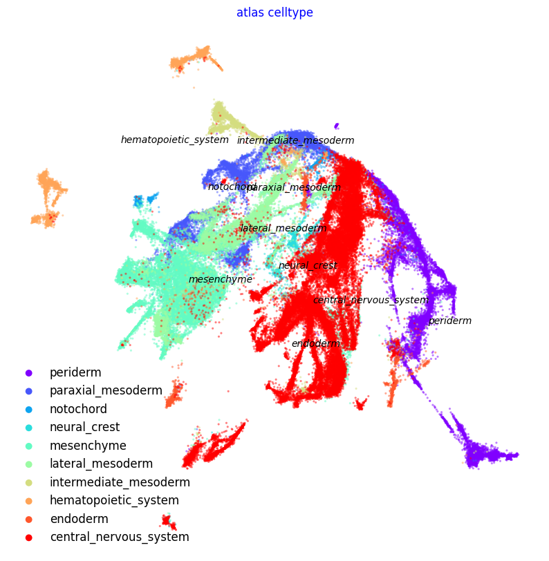
Plot Atlas Embedding’
print(f'{datetime.now()}\tPlot Atlas Embedding')
f1, ax = via.plot_scatter(embedding=atlas_embedding, labels=time_point_numeric, cmap='plasma', s=5,
                          alpha=0.5, edgecolors='None',
                          title='atlas', text_labels=False)
f1.set_size_inches(10, 10)

f2, ax = via.plot_scatter(embedding=atlas_embedding, labels=coarse_cell_type, title='atlas celltype',
                          alpha=0.5, s=5)
f2.set_size_inches(10, 10)
plt.show()
No artists with labels found to put in legend. Note that artists whose label start with an underscore are ignored when legend() is called with no argument.
2024-02-06 17:02:03.305009 Plot Atlas Embedding


Atlas View Edges
Compute the edges and pass it onto the via_object to avoid recomputing each time you plot
print(f'{datetime.now()}\tStart Computing Atlas View')
dict_coarse = {'notochord':2.5, 'central_nervous_system':5.5,'neural_crest':4.5,'paraxial_mesoderm':0,'intermediate_mesoderm':1,'lateral_mesoderm':1.5,
                       'mesenchyme':2.0,'hematopoietic_system':0.5,'periderm':8,'endoderm':7}
decay = 0.55#0.7  # increasing decay increasing merging of edges
i_bw = 0.035#0.05  # increasing bw increases merging of edges
global_visual_pruning = 0.55
n_milestones = 300

hammerbundle_dict = via.make_edgebundle_milestone(via_object=v0, n_milestones=n_milestones, decay=decay,
                                                  initial_bandwidth=i_bw,
                                                  global_visual_pruning=global_visual_pruning,
                                                  sc_labels_numeric=time_point_numeric)
v0.hammerbundle_milestone_dict = hammerbundle_dict  # make the hmbd in one shot to be used for all plots
2024-02-06 17:02:15.718628	Start Computing Atlas View
2024-02-06 17:02:15.718628	Start finding milestones
2024-02-06 17:02:50.911185	End milestones with 300
2024-02-06 17:02:52.349099	Recompute weights
2024-02-06 17:02:52.414034	pruning milestone graph based on recomputed weights
2024-02-06 17:02:52.417055	Graph has 1 connected components before pruning
2024-02-06 17:02:52.419138	Graph has 1 connected components after pruning
2024-02-06 17:02:52.419138	Graph has 1 connected components after reconnecting
2024-02-06 17:02:52.425153	regenerate igraph on pruned edges
2024-02-06 17:02:52.757955	Setting numeric label as time_series_labels or other sequential metadata for coloring edges
2024-02-06 17:02:53.431797	Making smooth edges
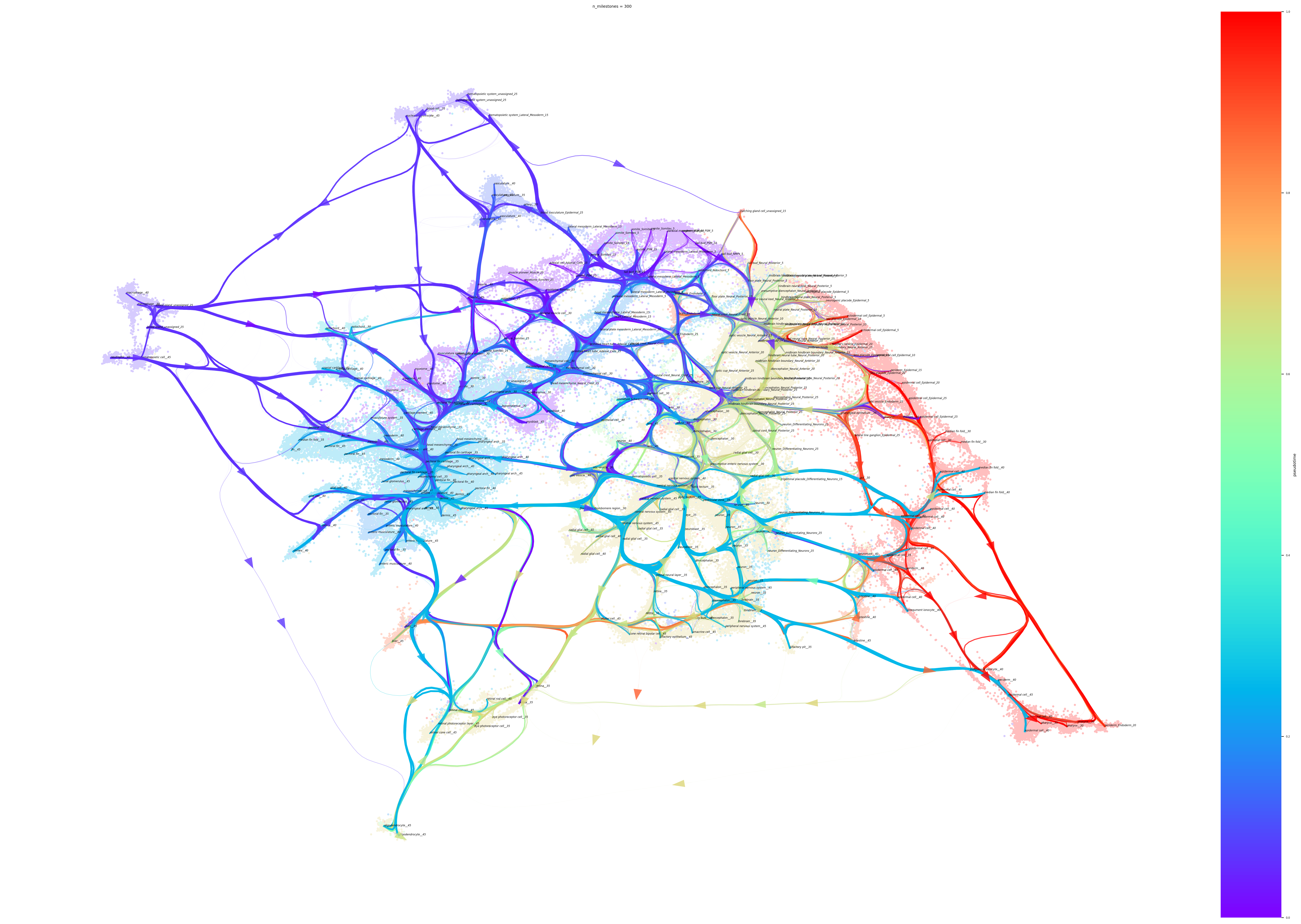
print(f'{datetime.now()}\tPlot Atlas View')
# color by tissue type, we
color_dict = {'notochord': 2.5, 'central_nervous_system': 5.5, 'neural_crest': 4.5, 'paraxial_mesoderm': 0,
               'intermediate_mesoderm': 1, 'lateral_mesoderm': 1.5,
               'mesenchyme': 2.0, 'hematopoietic_system': 0.5, 'periderm': 8, 'endoderm': 7}

#color by major cell type
headwidth_bundle = 0.2
fig, ax = via.plot_atlas_view(via_object=v0, sc_labels=hybrid_cell_time, fontsize_labels=4, text_labels=True,
                              add_sc_embedding=True, sc_scatter_alpha=0.25, sc_scatter_size=5,
                              cmap='rainbow', linewidth_bundle=3,
                              sc_labels=coarse_cell_type,
                              headwidth_bundle=headwidth_bundle)
fig.set_size_inches(35, 25)

plt.show()
2024-02-06 17:03:23.164984	Plot Atlas View
inside add sc embedding second if

#if you want to color by categories (e.g. tissue type)
#autogenerate color_dict
#color_dict = {}
#set_labels = list(set(labels))
#set_labels.sort(reverse=True)
#for index, value in enumerate(set_labels): color_dict[value] = index

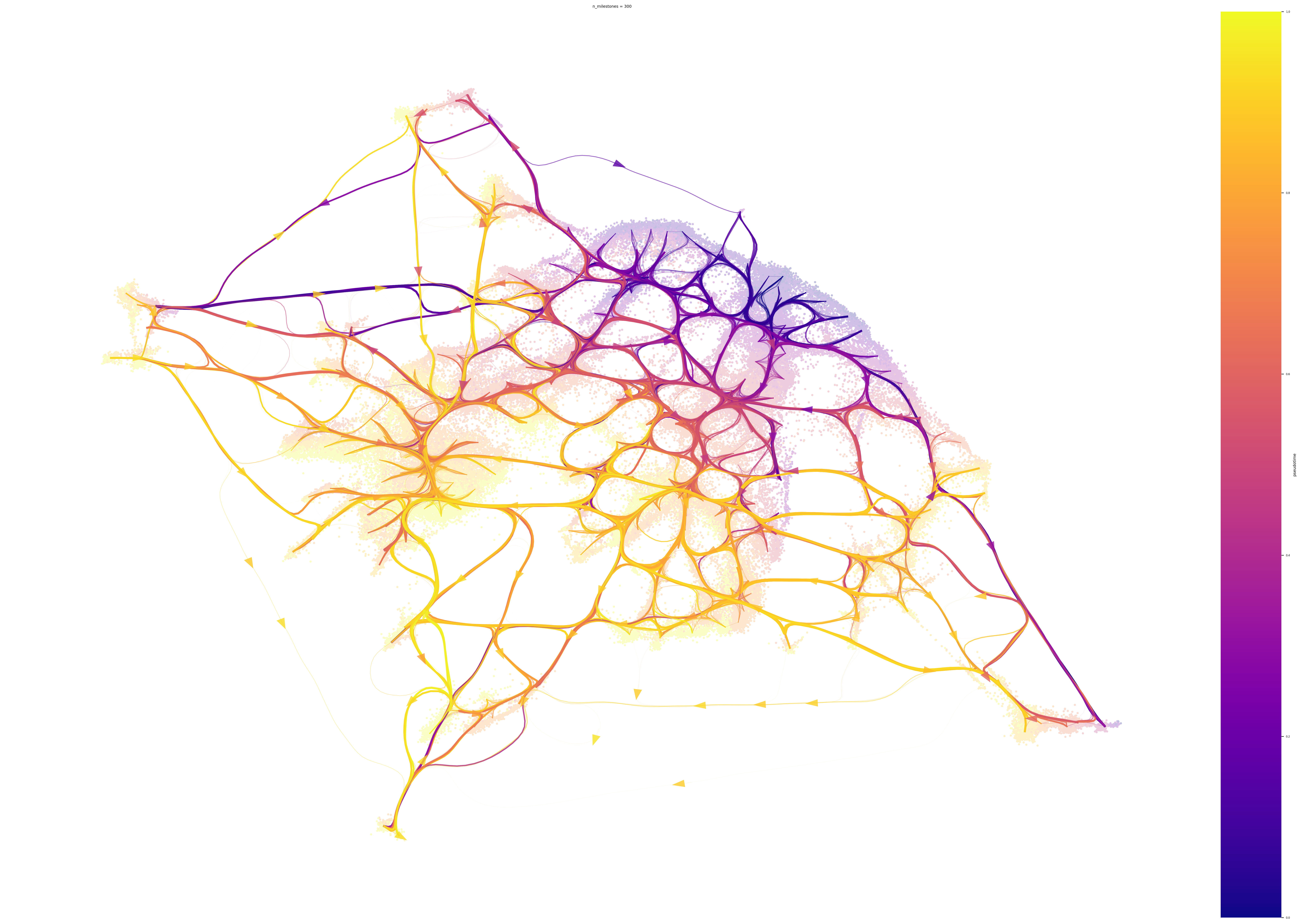
#color by stage
fig2, ax2 = via.plot_atlas_view(via_object=v0, sc_labels=hybrid_cell_time, fontsize_labels=2, text_labels=False,
                                add_sc_embedding=True, sc_scatter_alpha=0.25, sc_scatter_size=5, cmap='plasma',
                                sc_labels_expression=time_point_numeric,
                                linewidth_bundle=3,
                                headwidth_bundle=headwidth_bundle)
fig2.set_size_inches(35, 25)
inside add sc embedding second if
