API

Import pyvia as:

import pyVIA.core as via

API

• pyVIA core
• Plotting
• Util Functions for plotting
• Datasets

Full API

pyVIA core

class VIA.core.VIA(data, true_label=None, edgepruning_clustering_resolution_local=1, edgepruning_clustering_resolution=0.15, labels=None, keep_all_local_dist='auto', too_big_factor=0.4, resolution_parameter=1.0, partition_type='ModularityVP', small_pop=10, jac_weighted_edges=True, knn=30, n_iter_leiden=5, random_seed=42, num_threads=-1, distance='l2', time_smallpop=15, super_cluster_labels=False, super_node_degree_list=False, super_terminal_cells=False, x_lazy=0.99, alpha_teleport=0.99, root_user=None, preserve_disconnected=True, dataset='', super_terminal_clusters=[], is_coarse=True, csr_full_graph='', csr_array_locally_pruned='', ig_full_graph='', full_neighbor_array='', full_distance_array='', embedding=None, df_annot=None, preserve_disconnected_after_pruning=False, secondary_annotations=None, pseudotime_threshold_TS=30, cluster_graph_pruning=0.15, visual_cluster_graph_pruning=0.15, neighboring_terminal_states_threshold=3, num_mcmc_simulations=1300, piegraph_arrow_head_width=0.1, piegraph_edgeweight_scalingfactor=1.5, max_visual_outgoing_edges=2, via_coarse=None, velocity_matrix=None, gene_matrix=None, velo_weight=0.5, edgebundle_pruning=None, A_velo=None, CSM=None, edgebundle_pruning_twice=False, pca_loadings=None, time_series=False, time_series_labels=None, knn_sequential=10, knn_sequential_reverse=0, t_diff_step=1, single_cell_transition_matrix=None, embedding_type='via-mds', do_compute_embedding=False, color_dict=None, user_defined_terminal_cell=[], user_defined_terminal_group=[], do_gaussian_kernel_edgeweights=False, RW2_mode=False, working_dir_fp='/home/', memory=5, viagraph_decay=0.9, p_memory=1, graph_init_pos=None, spatial_coords=None, do_spatial_knn=False, do_spatial_layout=False, spatial_knn=15, spatial_aux=[])

A class to represent the VIA analysis

Parameters:

• data (ndarray) – input matrix of size n_cells x n_dims. Expects the PCs or features that will be used in the TI computation. Can be e.g. adata.obsm[‘X_pca][:,0:20]

• true_label (list) – list of str/int that correspond to the ground truth or reference annotations. Can also be None when no labels are available

• labels (ndarray (nsamples, )) – default is None. and PARC clusters are used for the viagraph. alternatively provide a list of clustermemberships that are integer values (not strings) to construct the viagraph using another clustering method or available annotations

• edgepruning_clustering_resolution_local (float) – default = 2 local level of pruning for PARC graph clustering stage. Range (0.1,3) higher numbers mean more edge retention. For large datasets can stick to just tuning edgepruning_clustering_resolution

• edgepruning_clustering_resolution (float) – (optional, default = 0.15, can also set as ‘median’) graph pruning for PARC clustering stage. Higher value keeps more edges, results in fewer clusters. Smaller value removes more edges and results in more clusters. Number of standard deviations below the network’s mean-jaccard-weighted edges. 0.1-1 provide reasonable pruning. higher value means less pruning (more edges retained). e.g. a value of 0.15 means all edges that are above mean(edgeweight)-0.15*std(edge-weights) are retained. We find both 0.15 and ‘median’ to yield good results/starting point and resulting in pruning away ~ 50-60% edges

• keep_all_local_dist (bool, str) – default value of ‘auto’ means that for smaller datasets local-pruning is done prior to clustering, but for large datasets local pruning is set to False for speed. can also set to be bool of True or False

• too_big_factor (float) – (optional, default=0.4). Forces clusters > 0.4*n_cells to be re-clustered

• resolution_parameter (float) – (default =1) larger value means more and smaller clusters

• partition_type (str) – (default “ModularityVP”) Options

• small_pop (int) – (default 10) Via attempts to merge Clusters with a population < 10 cells with larger clusters. If you have a very small dataset (e.g. few hundred cells), then consider lowering to e.g. 5

• jac_weighted_edges (bool) – (default = True) Use weighted edges in the PARC clustering step

• knn (int) – (optional, default = 30) number of K-Nearest Neighbors for HNSWlib KNN graph. Larger knn means more graph connectivity. Lower knn means more loosely connected clusters/cells

• n_iter_leiden (int) –

• random_seed (int) – Random seed to pass to clustering

• num_threads –

• distance (str) – (default ‘l2’) Euclidean distance ‘l2’ by default; other options ‘ip’ and ‘cosine’ for graph construction and similarity

• visual_cluster_graph_pruning (float) – (optional, default = 0.15) This only comes into play if the user deliberately chooses not to use the default edge-bundling method of visualizating edges (draw_piechart_graph()) and instead calls draw_piechart_graph_nobundle(). It is often set to the same value as the PARC clustering level of edgepruning_clustering_resolution. This does not impact computation of terminal states, pseudotime or lineage likelihoods. It controls the number of edges plotted for visual effect

• cluster_graph_pruning (float) – (optional, default =0.15) Pruning level of the cluster graph (does not impact number of clusters). Only impacts the connectivity of the clustergraph. Often set to the same value as the PARC clustering level of edgepruning_clustering_resolution.Reasonable range [0.1,1] To retain more connectivity in the clustergraph underlying the trajectory computations, increase the value

• time_smallpop (max time to be allowed handling singletons) –

• x_lazy (float) – (default =0.95) 1-x = probability of staying in same node (lazy). Values between 0.9-0.99 are reasonable

• alpha_teleport (float) – (default = 0.99) 1-alpha is probability of jumping. Values between 0.95-0.99 are reasonable unless prior knowledge of teleportation

• root_user (list, None) – can be a list of strings, a list of int or None (default is None) When the root_user is set as None and an RNA velocity matrix is available, a root will be automatically computed if the root_user is None and not velocity matrix is provided, then an arbitrary root is selected if the root_user is [‘celltype_earlystage’] where the str corresponds to an item in true_label, then a suitable starting point will be selected corresponding to this group if the root_user is [678], where 678 is the index of the cell chosen as a start cell, then this will be the designated starting cell. It is possible to give a list of root indices and groups. [120, 699] or [‘traj1_earlystage’, ‘traj2_earlystage’] when there are more than one trajectories

• preserve_disconnected (bool) – (default = True) If you believe there may be disconnected trajectories then set this to False

• dataset (str) – Can be set to ‘group’ or ‘’ (default). this refers to the type of root label (group level root or single cell index) you are going to provide. if your true_label has a sensible group of cells for a root then you can set dataset to ‘group’ and make the root parameter [‘labelname_root_cell_type’] if your root corresponds to one particular cell then set dataset = ‘’ (default)

• embedding (ndarray) – (optional, default = None) embedding (e.g. precomputed tsne, umap, phate, via-umap) for plotting data. Size n_cells x 2 If an embedding is provided when running VIA, then a scatterplot colored by pseudotime, highlighting terminal fates

• velo_weight (float) – (optional, default = 0.5) #float between [0,1]. the weight assigned to directionality and connectivity derived from scRNA-velocity

• neighboring_terminal_states_threshold (int) – (default = 3). Candidates for terminal states that are neighbors of each other may be removed from the list if they have this number of more of terminal states as neighbors

• knn_sequential (int) – (default =10) number of knn in the adjacent time-point for time-series data (t_i and t_i+1)

• knn_sequential_reverse (int) – (default = 0) number of knn enforced from current to previous time point

• t_diff_step (int) – (default =1) Number of permitted temporal intervals between connected nodes. If time data is labeled as [0,25,50,75,100,..] then t_diff_step=1 corresponds to ‘25’ and only edges within t_diff_steps are retained

• is_coarse (bool) – (default = True) If running VIA in two iterations where you wish to link the second fine-grained iteration with the initial iteration, then you set to False

• via_coarse (VIA) – (default = None) If instantiating a second iteration of VIA that needs to be linked to a previous iteration (e.g. via0), then set via_coarse to the previous via0 object

• df_annot (DataFrame) – (default None) used for the Mouse Organ data

• preserve_disconnected_after_pruning (bool) – (default = False) If you believe there are disconnected trajectories then set this to True and test your hypothesis

• A_velo (ndarray) – Cluster Graph Transition matrix based on rna velocity [n_clus x n_clus]

• velocity_matrix (matrix) – (default None) matrix of size [n_samples x n_genes]. this is the velocity matrix computed by scVelo (or similar package) and stored in adata.layers[‘velocity’]. The genes used for computing velocity should correspond to those useing in gene_matrix Requires gene_matrix to be provided too.

• gene_matrix (matrix) – (default None) Only used if Velocity_matrix is available. matrix of size [n_samples x n_genes]. We recommend using a subset like HVGs rather than full set of genes. (need to densify input if taking from adata = adata.X.todense())

• time_series (bool) – (default False) if the data has time-series labels then set to True

• time_series_labels (list) – (default None) list of integer values of temporal annoataions corresponding to e.g. hours (post fert), days, or sequential ordering

• pca_loadings (array) – (default None) the loadings of the pcs used to project the cells (to projected euclidean location based on velocity). n_cells x n_pcs

• secondary_annotations (None) – (default None)

• edgebundle_pruning (float) – (default=None) will by default be set to the same as the cluster_graph_pruning and influences the visualized level of pruning of edges. Typical values can be between [0,1] with higher numbers retaining more edges

• edgebundle_pruning_twice (bool) –

  default: False. When True, the edgebundling is applied to a further visually pruned (visual_cluster_graph_pruning) and can sometimes simplify the visualization. it does not impact the pseudotime and lineage computations piegraph_arrow_head_width: float

  (default = 0.1) size of arrow heads in via cluster graph

• piegraph_edgeweight_scalingfactor – (defaulf = 1.5) scaling factor for edge thickness in via cluster graph

• max_visual_outgoing_edges (int) – (default =2) Only allows max_visual_outgoing_edges to come out of any given node. Used in differentiation_flow()

• edgebundle_pruning – (default=None) will by default be set to the same as the cluster_graph_pruning and influences the visualized level of pruning of edges. Typical values can be between [0,1] with higher numbers retaining more edges

• edgebundle_pruning_twice – default: False. When True, the edgebundling is applied to a further visually pruned (visual_cluster_graph_pruning) and can sometimes simplify the visualization for very cluttered graphs. it does not impact the pseudotime and lineage computations

• pseudotime_threshold_TS (int) – (default = 30) corresponds to the criteria for a state to be considered a candidate terminal cell fate to be 30% or later of the computed psuedotime range

• num_mcmc_simulations (int) – (default = 1300) number of random walk simulations conducted

• embedding_type (str) – (default = ‘via-mds’, other options are ‘via-atlas’ and ‘via-force’

• do_compute_embedding (bool) – (default = False) If you want an embedding (n_samples x2) to be computed on the basis of the via sc graph then set this to True

• do_gaussian_kernel_edgeweights (bool) – (default = False) Type of edgeweighting on the graph edges

• memory (1/q * edge weight to a next-node that is not a neighbor of previous node. larger number means more memory and more introspective walk. small number <1 means more exploration) – (default = 2) higher q means more memory, more retrospective/inwards randomwalk. memory = 2 means run using the non-memory Via 1.0 mode

• viagraph_decay (float) – (default = 0.9) increasing decay causes more edges to merge

• memory –

• p_memory (1/p * edge weight to next node = previous node. large value means more exploration) –

• graph_init_pos (matrix (or list of lists) to initialize the viagraph) –

• spatial_coords (np.ndarray of size n_cells x 2 (denoting x,y coordinates) of each spot/cell) –

• do_spatial_knn (Whether or not to do spatial mode of StaVia for graph augmentation) –

• do_spatial_layout (whether to use spatial coords for layout of the clustergraph) –

• spatial_knn (int = 15. number of knn's added based on spatial proximity indiciated by spatial_coords) –

• spatial_aux (list = [] a list of slice IDs so that only cells/spots on the same slice are considered when building the spatial_knn graph) –

labels

length (n_samples, ) of cluster labels ndarray pre determined cluster labels user defined. #np.asarray(pre_labels).flatten()

Type:

array

single_cell_pt_markov

length n_samples of pseudotime

Type:

list

single_cell_bp

[n_lineages x n_samples] array of single cell branching probabilities towards each lineage (lineage normalized). Each column corresponds to a terminal state, in the order presented by the terminal_clusters attribute

Type:

ndarray

single_cell_bp_rownormed

[n_lineages x n_samples] array of single cell branching probabilities towards each lineage (cell normalized). Each column corresponds to a terminal state, in the order presented by the terminal_clusters attribute

Type:

ndarray

terminal_clusters

list of clusters that are cell fates/ unique lineages

Type:

list

cluster_bp

[n_clusters x n_terminal_states]. Lineage probability of cluster towards a particular terminal cluster state

Type:

ndarray

CSM

[n_cluster x n_clusters] array of cosine similarity used to weight the cluster graph transition matrix by velocity

Type:

ndarray

single_cell_transition_matrix

[n_samples x n_samples]

Type:

ndarray

terminal_clusters

(default None) list of terminal clusters

Type:

list

csr_full_graph

Type:

csr matrix of single-cell graph (augmented with sequential data when providing time_series information)

csr_array_locally_pruned

Type:

csr matrix

ig_full_graph

full_neighbor_array

user_defined_terminal_cell

Type:

list=[]

user_defined_terminal_group

Type:

list=[]

n_milestones

Type:

int = None Number of milestones in the via-mds computation (anything more than 10,000 can be computationally heavy and time consuming) Typically auto-determined within the via-mds function

embedding

[n_cells x 2] provided by user or autocomputed with via-mds or via-umap

Type:

ndarray

sc_transition_matrix(smooth_transition, b=10, use_sequentially_augmented=False)

#computes the single cell level transition directions that are later used to calculate velocity of embedding #based on changes at single cell level in genes and single cell level velocity

Parameters:

• smooth_transition –

• b – slope of logistic function

Returns:

Plotting

VIA.plotting_via.animate_atlas(hammerbundle_dict=None, via_object=None, linewidth_bundle=2, frame_interval=10, n_milestones=None, facecolor='white', cmap='plasma_r', extra_title_text='', size_scatter=1, alpha_scatter=0.2, saveto='/home/user/Trajectory/Datasets/animation_default.gif', time_series_labels=None, lineage_pathway=[], sc_labels_numeric=None, show_sc_embedding=False, sc_emb=None, sc_size_scatter=10, sc_alpha_scatter=0.2, n_intervals=50, n_repeat=2)

Parameters:

• ax – axis to plot on

• hammer_bundle – hammerbundle object with coordinates of all the edges to draw

• layout – coords of cluster nodes and optionally also contains the numeric value associated with each cluster (such as time-stamp) layout[[‘x’,’y’,’numeric label’]] sc/cluster/milestone level

• CSM – cosine similarity matrix. cosine similarity between the RNA velocity between neighbors and the change in gene expression between these neighbors. Only used when available

• velocity_weight – percentage weightage given to the RNA velocity based transition matrix

• pt – cluster-level pseudotime

• alpha_bundle – alpha when drawing lines

• linewidth_bundle – linewidth of bundled lines

• edge_color –

• frame_interval (int) – smaller number, faster refresh and video

• facecolor (str) – default = white

• headwidth_bundle – headwidth of arrows used in bundled edges

• arrow_frequency – min dist between arrows (bundled edges otherwise have overcrowding of arrows)

• show_direction – True will draw arrows along the lines to indicate direction

• milestone_edges – pandas DataFrame milestone_edges[[‘source’,’target’]]

:param t_diff_factor scaling the average the time intervals (0.25 means that for each frame, the time is progressed by 0.25* mean_time_differernce_between adjacent times (only used when sc_labels_numeric are directly passed instead of using pseudotime) :type show_sc_embedding: bool :param show_sc_embedding: plot the single cell embedding under the edges :param sc_emb numpy array of single cell embedding (ncells x 2) :param sc_alpha_scatter, Alpha transparency value of points of single cells (1 is opaque, 0 is fully transparent) :param sc_size_scatter. size of scatter points of single cells :param n_repeat. number of times you repeat the whole process :return: axis with bundled edges plotted

VIA.plotting_via.animate_atlas_old(hammerbundle_dict=None, via_object=None, linewidth_bundle=2, frame_interval=10, n_milestones=None, facecolor='white', cmap='plasma_r', extra_title_text='', size_scatter=1, alpha_scatter=0.2, saveto='/home/user/Trajectory/Datasets/animation_default.gif', time_series_labels=None, lineage_pathway=[], sc_labels_numeric=None, t_diff_factor=0.25, show_sc_embedding=False, sc_emb=None, sc_size_scatter=10, sc_alpha_scatter=0.2, n_intervals=50)

Parameters:

• ax – axis to plot on

• hammer_bundle – hammerbundle object with coordinates of all the edges to draw

• layout – coords of cluster nodes and optionally also contains the numeric value associated with each cluster (such as time-stamp) layout[[‘x’,’y’,’numeric label’]] sc/cluster/milestone level

• CSM – cosine similarity matrix. cosine similarity between the RNA velocity between neighbors and the change in gene expression between these neighbors. Only used when available

• velocity_weight – percentage weightage given to the RNA velocity based transition matrix

• pt – cluster-level pseudotime

• alpha_bundle – alpha when drawing lines

• linewidth_bundle – linewidth of bundled lines

• edge_color –

• frame_interval (int) – smaller number, faster refresh and video

• facecolor (str) – default = white

• headwidth_bundle – headwidth of arrows used in bundled edges

• arrow_frequency – min dist between arrows (bundled edges otherwise have overcrowding of arrows)

• show_direction – True will draw arrows along the lines to indicate direction

• milestone_edges – pandas DataFrame milestone_edges[[‘source’,’target’]]

:param t_diff_factor scaling the average the time intervals (0.25 means that for each frame, the time is progressed by 0.25* mean_time_differernce_between adjacent times (only used when sc_labels_numeric are directly passed instead of using pseudotime) :type show_sc_embedding: bool :param show_sc_embedding: plot the single cell embedding under the edges :param sc_emb numpy array of single cell embedding (ncells x 2) :param sc_alpha_scatter, Alpha transparency value of points of single cells (1 is opaque, 0 is fully transparent) :param sc_size_scatter. size of scatter points of single cells :param time_series_labels, should be a single-cell level list (n_cells) of numerical values that form a discrete set. I.e. not continuous like pseudotime, :return: axis with bundled edges plotted

VIA.plotting_via.animate_streamplot(via_object, embedding, density_grid=1, linewidth=0.5, min_mass=1, cutoff_perc=None, scatter_size=500, scatter_alpha=0.2, marker_edgewidth=0.1, smooth_transition=1, smooth_grid=0.5, color_scheme='annotation', other_labels=[], b_bias=20, n_neighbors_velocity_grid=None, fontsize=8, alpha_animate=0.7, cmap_scatter='rainbow', cmap_stream='Blues', segment_length=1, saveto='/home/shobi/Trajectory/Datasets/animation.gif', use_sequentially_augmented=False, facecolor_='white', random_seed=0)

Draw Animated vector plots. the Saved .gif file saved at the saveto address, is the best for viewing the animation as the fig, ax output can be slow

Parameters:

• via_object – viaobject

• embedding – ndarray (nsamples,2) umap, tsne, via-umap, via-mds

• density_grid –

• linewidth –

• min_mass –

• cutoff_perc –

• scatter_size –

• scatter_alpha –

• marker_edgewidth –

• smooth_transition –

• smooth_grid –

• color_scheme – ‘annotation’, ‘cluster’, ‘other’

• add_outline_clusters –

• cluster_outline_edgewidth –

• gp_color –

• bg_color –

• title –

• b_bias –

• n_neighbors_velocity_grid –

• fontsize –

• alpha_animate –

• cmap_scatter –

• cmap_stream – string of a cmap for streamlines, default = ‘Blues’ (for dark blue lines) . Consider ‘Blues_r’ for white lines OR ‘Greys/_r’ ‘gist_yard/_r’

• color_stream – string like ‘white’. will override cmap_stream

• segment_length –

Returns:

fig, ax.

VIA.plotting_via.get_gene_expression(via_object, gene_exp, cmap='jet', dpi=150, marker_genes=[], linewidth=2.0, n_splines=10, spline_order=4, fontsize_=8, marker_lineages=[], optional_title_text='', cmap_dict=None)

Parameters:

• via_object – via object

• gene_exp (DataFrame) – dataframe where columns are features (gene) and rows are single cells

• cmap (str) – default: ‘jet’

• dpi (int) – default:150

• marker_genes (list) – Default is to use all genes in gene_exp. other provide a list of marker genes that will be used from gene_exp.

• linewidth (float) – default:2

• n_slines – default:10 Note n_splines must be > spline_order.

• spline_order (int) – default:4 n_splines must be > spline_order.

• marker_lineages – Default is to use all lineage pathways. other provide a list of lineage number (terminal cluster number).

• cmap_dict (dict) – {lineage number: ‘color’}

Returns:

fig, axs

VIA.plotting_via.make_dict_of_clusters_for_each_celltype(via_labels=[], true_label=[], verbose=False)

Parameters:

• via_labels (list) – usually set to via_object.labels. list of length n_cells of cluster membership

• true_label (list) – cell type labels (list of length n_cells)

Returns:

VIA.plotting_via.make_edgebundle_milestone(embedding=None, sc_graph=None, via_object=None, sc_pt=None, initial_bandwidth=0.03, decay=0.7, n_milestones=None, milestone_labels=[], sc_labels_numeric=None, weighted=True, global_visual_pruning=0.5, terminal_cluster_list=[], single_cell_lineage_prob=None, random_state=0)

Perform Edgebundling of edges in a milestone level to return a hammer bundle of milestone-level edges. This is more granular than the original parc-clusters but less granular than single-cell level and hence also less computationally expensive requires some type of embedding (n_samples x 2) to be available

Parameters:

• embedding (ndarray) – optional (not required if via_object is provided) embedding single cell. also looks nice when done on via_mds as more streamlined continuous diffused graph structure. Umap is a but “clustery”

• graph – optional (not required if via_object is provided) igraph single cell graph level

• via_object – via_object (best way to run this function by simply providing via_object)

• sc_graph – igraph graph set as the via attribute self.ig_full_graph (affinity graph)

• initial_bandwidth – increasing bw increases merging of minor edges

• decay – increasing decay increases merging of minor edges #https://datashader.org/user_guide/Networks.html

• milestone_labels (list) – default list=[]. Usually autocomputed. but can provide as single-cell level labels (clusters, groups, which function as milestone groupings of the single cells)

• sc_labels_numeric (list) – default is None which automatically chooses via_object’s pseudotime or time_series_labels (when available). otherwise set to a list of numerical values representing some sequential/chronological information

• terminal_cluster_list (list) – default list [] and automatically uses all terminal clusters. otherwise set to any of the terminal cluster numbers within a list

Returns:

dictionary containing keys: hb_dict[‘hammerbundle’] = hb hammerbundle class with hb.x and hb.y containing the coords hb_dict[‘milestone_embedding’] dataframe with ‘x’ and ‘y’ columns for each milestone and hb_dict[‘edges’] dataframe with columns [‘source’,’target’] milestone for each each and [‘cluster_pop’], hb_dict[‘sc_milestone_labels’] is a list of milestone label for each single cell

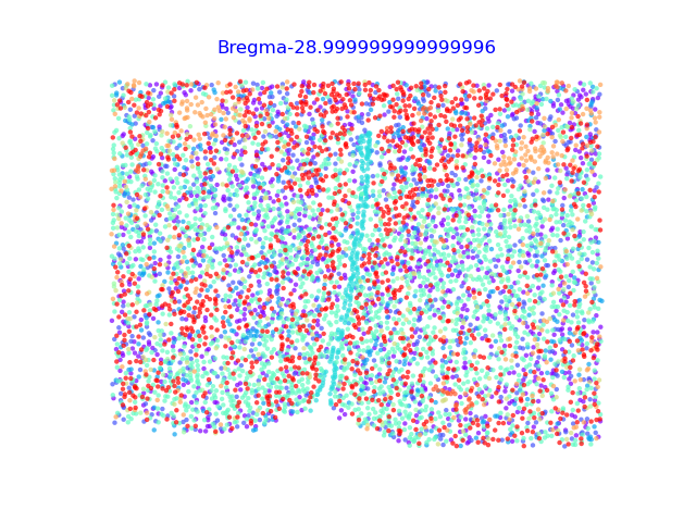
VIA.plotting_via.plot_all_spatial_clusters(spatial_coords, true_label, via_labels, save_to='', color_dict={}, cmap='rainbow', alpha=0.4, s=5, verbose=False, reference_labels=[], reference_labels2=[])

Parameters:

• spatial_coords – ndarray of x,y coords of tissue location of cells (ncells x2)

• true_label – categorial labels (list of length n_cells)

• via_labels – cluster membership labels (list of length n_cells)

• save_to (str) –

• color_dict (dict) – optional dict with keys corresponding to true_label type. e.g. {true_label_celltype1: ‘green’,true_label_celltype2: ‘red’}

• cmap (str) – string default = rainbow

• reference_labels (list) – optional list of single-cell labels (e.g. time, annotation). Used to selectively provide a grey background to cells not in the cluster being inspected. If you have multipe time points, then set reference_labels to the time_points. All cells in the most prevalent timepoint seen in the cluster of interest will be plotted as a background

• reference_labels2 (list) – optional list of single-cell labels (e.g. time, annotation). this will be used in the title of each subplot to note the majority cell (ref2) type for each cluster

Returns:

list lists of [[fig1, axs_set1], [fig2, axs_set2],…]

VIA.plotting_via.plot_atlas_view(hammerbundle_dict=None, via_object=None, alpha_bundle_factor=1, linewidth_bundle=2, facecolor='white', cmap='plasma', extra_title_text='', alpha_milestones=0.3, headwidth_bundle=0.1, headwidth_alpha=0.8, arrow_frequency=0.05, show_arrow=True, sc_labels_sequential=None, sc_labels_expression=None, initial_bandwidth=0.03, decay=0.7, n_milestones=None, scale_scatter_size_pop=False, show_milestones=True, sc_labels=None, text_labels=False, lineage_pathway=[], dpi=300, fontsize_title=6, fontsize_labels=6, global_visual_pruning=0.5, use_sc_labels_sequential_for_direction=False, sc_scatter_size=3, sc_scatter_alpha=0.4, add_sc_embedding=True, size_milestones=5, colorbar_legend='pseudotime')

Edges can be colored by time-series numeric labels, pseudotime, lineage pathway probabilities, or gene expression. If not specificed then time-series is chosen if available, otherwise falls back to pseudotime. to use gene expression the sc_labels_expression is provided as a list. To specify other numeric sequential data provide a list of sc_labels_sequential = [] n_samples in length. via_object.embedding must be an ndarray of shape (nsamples,2)

Parameters:

• hammer_bundle_dict – dictionary with keys: hammerbundle object with coordinates of all the edges to draw. If hammer_bundle and layout are None, then this will be computed internally

• via_object – type via object, if hammerbundle_dict is None, then you must provide a via_object. Ensure that via_object has embedding attribute

• layout – coords of cluster nodes and optionally also contains the numeric value associated with each cluster (such as time-stamp) layout[[‘x’,’y’,’numeric label’]] sc/cluster/milestone level

• CSM – cosine similarity matrix. cosine similarity between the RNA velocity between neighbors and the change in gene expression between these neighbors. Only used when available

• velocity_weight – percentage weightage given to the RNA velocity based transition matrix

• pt – cluster-level pseudotime

• alpha_bundle – alpha when drawing lines

• linewidth_bundle – linewidth of bundled lines

• edge_color –

• alpha_milestones (float) – float 0.3 alpha of milestones

• size_milestones (int) – scatter size of the milestones (use sc_size_scatter to control single cell scatter when using in conjunction with lineage probs/ sc embeddings)

• arrow_frequency (float) – min dist between arrows (bundled edges otherwise have overcrowding of arrows)

• show_direction – True will draw arrows along the lines to indicate direction

• milestone_edges – pandas DataFrame milestoone_edges[[‘source’,’target’]]

• milestone_numeric_values – the milestone average of numeric values such as time (days, hours), location (position), or other numeric value used for coloring edges in a sequential manner if this is None then the edges are colored by length to distinguish short and long range edges

• arrow_frequency – 0.05. higher means fewer arrows

• n_milestones (int) – int None. if no hammerbundle_dict is provided, but via_object is provided, then the user can specify level of granularity by setting the n_milestones. otherwise it will be automatically selected

• scale_scatter_size_pop (bool) – bool default False

• sc_labels_expression (list) – list single cell numeric values used for coloring edges and nodes of corresponding milestones mean expression levels (len n_single_cell samples) edges can be colored by time-series numeric (gene expression)/string (cell type) labels, pseudotime, or gene expression. If not specificed then time-series is chosen if available, otherwise falls back to pseudotime. to use gene expression the sc_labels_expression is provided as a list

• sc_labels_sequential (list) – list single cell numeric sequential values used for directionality inference as replacement for pseudotime or via_object.time_series_labels (len n_samples single cell)

• sc_labels (list) – list None list of single-cell level labels (categorial or discrete set of numerical values) to label the nodes

• text_labels (bool) – bool False if you want to label the nodes based on sc_labels (or true_label if via_object is provided)

• lineage_pathway (list) – list of terminal states to plot lineage pathways

• use_sc_labels_sequential_for_direction (bool) – use the sequential data (timeseries labels or other provided by user) to direct the arrows

:param lineage_alpha_threshold number representing the percentile (0-100) of lineage likelikhood in a particular lineage pathway, below which edges will be drawn with lower alpha transparency factor :type sc_scatter_alpha: float :param sc_scatter_alpha: transparency of the background singlecell scatter when plotting lineages :type add_sc_embedding: bool :param add_sc_embedding: add background of single cell scatter plot for Atlas :param scatter_size_sc_embedding :param colorbar_legend str title of colorbar :return: fig, axis with bundled edges plotted

VIA.plotting_via.plot_clusters_spatial(spatial_coords, clusters=[], via_labels=[], title_sup='', fontsize_=6, color='green', s=5, alpha=0.5, xlim_max=None, ylim_max=None, xlim_min=None, ylim_min=None, reference_labels=[], reference_labels2=[], equal_axes_lim=True)

Parameters:

• spatial_coords – ndarray of spatial coords ncellsx2 dims

• clusters – the clusters in via_object.labels which you want to plot (usually a subset of the total number of clusters)

• via_labels – via_object.labels (cluster level labels, list of n_cells length)

• title_sup – title of the overall figure

• fontsize – fontsize for legend

• color – color of scatter points

• s (int) – size of scatter points

• alpha – float alpha transparency of scatter (0 fully transporent, 1 is opaque)

• xlim_max – limits of axes

• ylim_max – limits of axes

• xlim_min – limits of axes

• ylim_min – limits of axes

• reference_labels (list) – optional list of single-cell labels (e.g. time, annotation). this will be used in the title of each subplot to note the majority cell (ref2) type for each cluster

• reference_labels2 (list) – optional list of single-cell labels (e.g. time, annotation). this will be used in the title of each subplot to note the majority cell (ref2) type for each cluster

Returns:

fig, axs

VIA.plotting_via.plot_differentiation_flow(via_object, idx=None, dpi=150, marker_lineages=[], label_node=[], do_log_flow=True, fontsize=8, alpha_factor=0.9, majority_cluster_population_dict=None, cmap_sankey='rainbow', title_str='Differentiation Flow', root_cluster_list=None)

#SANKEY PLOTS G is the igraph knn (low K) used for shortest path in high dim space. no idx needed as it’s made on full sample knn_hnsw is the knn made in the embedded space used for query to find the nearest point in the downsampled embedding that corresponds to the single cells in the full graph

Parameters:

• via_object –

• embedding – n_samples x 2. embedding is 2D representation of the full dataset.

• idx (list) – if one uses a downsampled embedding of the original data, then idx is the selected indices of the downsampled samples used in the visualization

• cmap_name –

• dpi –

:param do_log_flow bool True (default) take the natural log (1+edge flow value) :param label_node list of labels for each cell (could be cell type, stage level) length is n_cells :param scatter_size: if None, then auto determined based on n_cells :param marker_lineages: Default is to use all lineage pathways. other provide a list of lineage number (terminal cluster number). :type alpha_factor: float :param alpha_factor: float transparency :type root_cluster_list: list :param root_cluster_list: list of roots by cluster number e.g. [5] means a good root is cluster number 5 :return: fig, axs

VIA.plotting_via.plot_gene_trend_heatmaps(via_object, df_gene_exp, marker_lineages=[], fontsize=8, cmap='viridis', normalize=True, ytick_labelrotation=0, fig_width=7)

Plot the gene trends on heatmap: a heatmap is generated for each lineage (identified by terminal cluster number). Default selects all lineages

Parameters:

• via_object –

• df_gene_exp (DataFrame) – pandas DataFrame single-cell level expression [cells x genes]

• marker_lineages (list) – list default = None and plots all detected all lineages. Optionally provide a list of integers corresponding to the cluster number of terminal cell fates

• fontsize (int) – int default = 8

• cmap (str) – str default = ‘viridis’

• normalize (bool) – bool = True

• ytick_labelrotation (int) – int default = 0

Returns:

fig and list of axes

VIA.plotting_via.plot_piechart_only_viagraph(via_object, type_data='pt', gene_exp=[], cmap_piechart='rainbow', title='', cmap=None, ax_text=True, dpi=150, headwidth_arrow=0.1, alpha_edge=0.4, linewidth_edge=2, edge_color='darkblue', reference_labels=None, show_legend=True, pie_size_scale=0.8, fontsize=8, pt_visual_threshold=99, highlight_terminal_clusters=True, size_node_notpiechart=1, tune_edges=False, initial_bandwidth=0.05, decay=0.9, edgebundle_pruning=0.5)

plot two subplots with a clustergraph level representation of the viagraph showing true-label composition (lhs) and pseudotime/gene expression (rhs) Returns matplotlib figure with two axes that plot the clustergraph using edge bundling left axis shows the clustergraph with each node colored by annotated ground truth membership. right axis shows the same clustergraph with each node colored by the pseudotime or gene expression

Parameters:

• via_object – is class VIA (the same function also exists as a method of the class and an external plotting function

• type_data – string default ‘pt’ for pseudotime colored nodes. or ‘gene’

• gene_exp (list) – list of values (or column of dataframe) corresponding to feature or gene expression to be used to color nodes at CLUSTER level

• cmap_piechart (str) – str cmap for piechart categories

• title – string

• cmap (str) – default None. automatically chooses coolwarm for gene expression or viridis_r for pseudotime

• ax_text – Bool default= True. Annotates each node with cluster number and population of membership

• dpi – int default = 150

• headwidth_arrow – default = 0.1. width of arrowhead used to directed edges

• reference_labels – None or list. list of categorical (str) labels for cluster composition of the piecharts (LHS subplot) length = n_samples.

• pie_size_scale (float) – float default=0.8 scaling factor of the piechart nodes

• pt_visual_threshold (int) – int (percentage) default = 95 corresponding to rescaling the visual color scale by clipping outlier cluster pseudotimes

:param highlight_terminal_clusters:bool = True (red border around terminal clusters) :type size_node_notpiechart: float :param size_node_notpiechart: scaling factor for node size of the viagraph (not the piechart part) :param initial_bandwidth: (float = 0.05) increasing bw increases merging of minor edges. Only used when tune_edges = True :param decay: (decay = 0.9) increasing decay increases merging of minor edges . Only used when tune_edges = True :param edgebundle_pruning (float = 0.5). takes on values between 0-1. smaller value means more pruning away edges that can be visualised. Only used when tune_edges = True :return: f, ax, ax1

VIA.plotting_via.plot_piechart_viagraph(via_object, type_data='pt', gene_exp=[], cmap_piechart='rainbow', title='', cmap=None, ax_text=True, dpi=150, headwidth_arrow=0.1, alpha_edge=0.4, linewidth_edge=2, edge_color='darkblue', reference_labels=None, show_legend=True, pie_size_scale=0.8, fontsize=8, pt_visual_threshold=99, highlight_terminal_clusters=True, size_node_notpiechart=1, tune_edges=False, initial_bandwidth=0.05, decay=0.9, edgebundle_pruning=0.5)

plot two subplots with a clustergraph level representation of the viagraph showing true-label composition (lhs) and pseudotime/gene expression (rhs) Returns matplotlib figure with two axes that plot the clustergraph using edge bundling left axis shows the clustergraph with each node colored by annotated ground truth membership. right axis shows the same clustergraph with each node colored by the pseudotime or gene expression

Parameters:

• via_object – is class VIA (the same function also exists as a method of the class and an external plotting function

• type_data – string default ‘pt’ for pseudotime colored nodes. or ‘gene’

• gene_exp (list) – list of values (or column of dataframe) corresponding to feature or gene expression to be used to color nodes at CLUSTER level

• cmap_piechart (str) – str cmap for piechart categories

• title – string

• cmap (str) – default None. automatically chooses coolwarm for gene expression or viridis_r for pseudotime

• ax_text – Bool default= True. Annotates each node with cluster number and population of membership

• dpi – int default = 150

• headwidth_arrow – default = 0.1. width of arrowhead used to directed edges

• reference_labels – None or list. list of categorical (str) labels for cluster composition of the piecharts (LHS subplot) length = n_samples.

• pie_size_scale (float) – float default=0.8 scaling factor of the piechart nodes

• pt_visual_threshold (int) – int (percentage) default = 95 corresponding to rescaling the visual color scale by clipping outlier cluster pseudotimes

:param highlight_terminal_clusters:bool = True (red border around terminal clusters) :type size_node_notpiechart: float :param size_node_notpiechart: scaling factor for node size of the viagraph (not the piechart part) :param initial_bandwidth: (float = 0.05) increasing bw increases merging of minor edges. Only used when tune_edges = True :param decay: (decay = 0.9) increasing decay increases merging of minor edges . Only used when tune_edges = True :param edgebundle_pruning (float = 0.5). takes on values between 0-1. smaller value means more pruning away edges that can be visualised. Only used when tune_edges = True :return: f, ax, ax1

VIA.plotting_via.plot_population_composition(via_object, time_labels=None, celltype_list=None, cmap='rainbow', legend=True, alpha=0.5, linewidth=0.2, n_intervals=20, xlabel='time', ylabel='', title='Cell populations', color_dict=None, fraction=True)

Parameters:

• via_object – optional. this is required unless both time_labels and cell_labels are provided as arguments to the function

• time_labels (list) – list length n_cells of pseudotime or known stage numeric labels

• cell_labels – list of cell type or cluster length n_cells

Returns:

ax

VIA.plotting_via.plot_sc_lineage_probability(via_object, embedding=None, idx=None, cmap_name='plasma', dpi=150, scatter_size=None, marker_lineages=[], fontsize=8, alpha_factor=0.9, majority_cluster_population_dict=None, cmap_sankey='rainbow', do_sankey=False)

G is the igraph knn (low K) used for shortest path in high dim space. no idx needed as it’s made on full sample knn_hnsw is the knn made in the embedded space used for query to find the nearest point in the downsampled embedding that corresponds to the single cells in the full graph

Parameters:

• via_object –

• embedding (ndarray) – n_samples x 2. embedding is either the full or downsampled 2D representation of the full dataset.

• idx (list) – if one uses a downsampled embedding of the original data, then idx is the selected indices of the downsampled samples used in the visualization

• cmap_name –

• dpi –

• scatter_size – if None, then auto determined based on n_cells

• marker_lineages – Default is to use all lineage pathways. other provide a list of lineage number (terminal cluster number).

• alpha_factor (float) – float transparency

Returns:

fig, axs

VIA.plotting_via.plot_scatter(embedding, labels, cmap='rainbow', s=5, alpha=0.3, edgecolors='None', title='', text_labels=True, color_dict=None, via_object=None, sc_index_terminal_states=None, true_labels=[], show_legend=True, hide_axes_ticks=True, color_labels_reverse=False)

General scatter plotting tool for numeric and categorical labels on the single-cell level

Parameters:

• embedding (ndarray) – ndarray n_samples x 2

• labels (list) – list single cell labels list of number or strings

• cmap – str default = ‘rainbow’

• s – int size of scatter dot

• alpha – float with 0 transparent to 1 opaque default =0.3

• edgecolors –

• title (str) – str

• text_labels (bool) – bool default =True

• via_object –

• sc_index_terminal_states (list) – list of integers corresponding to one cell in each of the terminal states

• color_dict – {‘true_label_group_1’: #COLOR,’true_label_group_2’: #COLOR2,….} where the dictionary keys correspond to the provided labels

• true_labels (list) – list of single cell labels used to annotate the terminal states

Returns:

matplotlib pyplot fig, ax

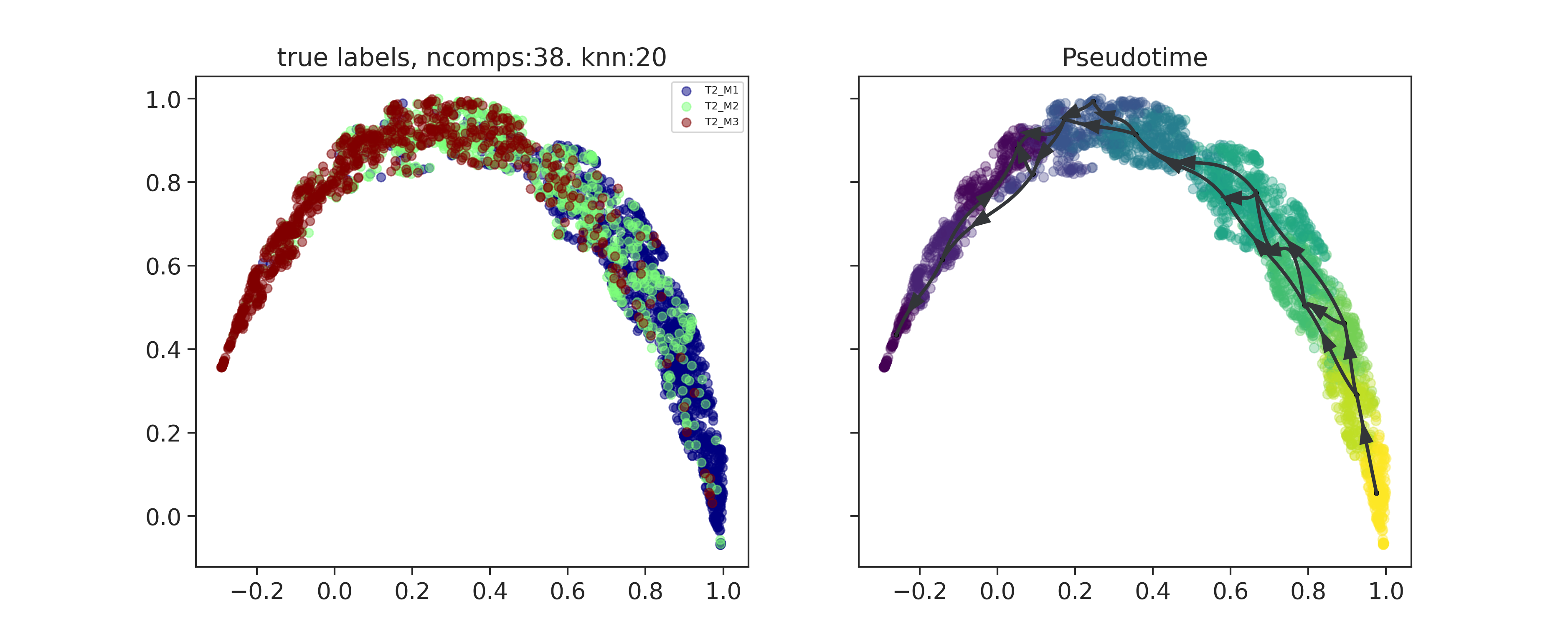
VIA.plotting_via.plot_trajectory_curves(via_object, embedding=None, idx=None, title_str='Pseudotime', draw_all_curves=True, arrow_width_scale_factor=15.0, scatter_size=50, scatter_alpha=0.5, linewidth=1.5, marker_edgewidth=1, cmap_pseudotime='viridis_r', dpi=150, highlight_terminal_states=True, use_maxout_edgelist=False)

projects the graph based coarse trajectory onto a umap/tsne embedding

Parameters:

• via_object – via object

• embedding (ndarray) – 2d array [n_samples x 2] with x and y coordinates of all n_samples. Umap, tsne, pca OR use the via computed embedding via_object.embedding

• idx (Optional[list]) – default: None. Or List. if you had previously computed a umap/tsne (embedding) only on a subset of the total n_samples (subsampled as per idx), then the via objects and results will be indexed according to idx too

• title_str (str) – title of figure

• draw_all_curves (bool) – if the clustergraph has too many edges to project in a visually interpretable way, set this to False to get a simplified view of the graph pathways

• arrow_width_scale_factor (float) –

• scatter_size (float) –

• scatter_alpha (float) –

• linewidth (float) –

• marker_edgewidth (float) –

• cmap_pseudotime (str) –

• dpi (int) – int default = 150. Use 300 for paper figures

• highlight_terminal_states (bool) – whether or not to highlight/distinguish the clusters which are detected as the terminal states by via

Returns:

f, ax1, ax2

VIA.plotting_via.plot_viagraph(via_object, type_data='gene', df_genes=None, gene_list=[], arrow_head=0.1, edgeweight_scale=1.5, cmap=None, label_text=True, size_factor_node=1, tune_edges=False, initial_bandwidth=0.05, decay=0.9, edgebundle_pruning=0.5)

cluster level expression of gene/feature intensity :param via_object: :param type_data: :param gene_exp: pd.Dataframe size n_cells x genes. Otherwise defaults to plotting pseudotime :type gene_list: list :param gene_list: list of gene names corresponding to the column name :type arrow_head: float :param arrow_head: :type edgeweight_scale: float :param edgeweight_scale: :param cmap: :type label_text: bool :param label_text: bool to add numeric values of the gene exp level :param size_factor_node size of graph nodes :type tune_edges: bool :param tune_edges: bool (false). if you want to change the number of edges visualized, then set this to True and modify the tuning parameters (initial_bandwidth, decay, edgebundle_pruning) :param initial_bandwidth: (float = 0.05) increasing bw increases merging of minor edges. Only used when tune_edges = True :param decay: (decay = 0.9) increasing decay increases merging of minor edges . Only used when tune_edges = True :param edgebundle_pruning (float = 0.5). takes on values between 0-1. smaller value means more pruning away edges that can be visualised. Only used when tune_edges = True :return: fig, axs

VIA.plotting_via.plot_viagraph_(ax=None, hammer_bundle=None, layout=None, CSM=None, velocity_weight=None, pt=None, alpha_bundle=1, linewidth_bundle=2, edge_color='darkblue', headwidth_bundle=0.1, arrow_frequency=0.05, show_direction=True, ax_text=True, title='', plot_clusters=False, cmap='viridis', via_object=None, fontsize=9, dpi=300, tune_edges=False, initial_bandwidth=0.05, decay=0.9, edgebundle_pruning=0.5)

this plots the edgebundles on the via clustergraph level and also adds the relevant arrow directions based on the TI directionality

Parameters:

• ax – axis to plot on

• hammer_bundle – hammerbundle object with coordinates of all the edges to draw. self.hammer

• layout (ndarray) – coords of cluster nodes

• CSM (ndarray) – cosine similarity matrix. cosine similarity between the RNA velocity between neighbors and the change in gene expression between these neighbors. Only used when available

• velocity_weight (float) – percentage weightage given to the RNA velocity based transition matrix

• pt (list) – cluster-level pseudotime (or other intensity level of features at average-cluster level)

• alpha_bundle – alpha when drawing lines

• linewidth_bundle – linewidth of bundled lines

• edge_color –

• headwidth_bundle – headwidth of arrows used in bundled edges

• arrow_frequency – min dist between arrows (bundled edges otherwise have overcrowding of arrows)

• show_direction – bool default True. will draw arrows along the lines to indicate direction

• plot_clusters (bool) – bool default False. When this function is called on its own (and not from within draw_piechart_graph() then via_object must be provided

• ax_text (bool) – bool default True. Show labels of the clusters with the cluster population and PARC cluster label

• fontsize (float) – float default 9 Font size of labels

Returns:

fig, ax with bundled edges plotted

VIA.plotting_via.via_atlas_emb(via_object=None, X_input=None, graph=None, n_components=2, alpha=1.0, negative_sample_rate=5, gamma=1.0, spread=1.0, min_dist=0.1, init_pos='via', random_state=0, n_epochs=100, distance_metric='euclidean', layout=None, cluster_membership=None, parallel=False, saveto='', n_jobs=2)

Run dimensionality reduction using the VIA modified HNSW graph using via cluster graph initialization when Via_object is provided

Parameters:

• via_object – if via_object is provided then X_input and graph are ignored

• X_input (ndarray) – ndarray nsamples x features (PCs)

• graph (csr_matrix) – csr_matrix of knngraph. This usually is via’s pruned, sequentially augmented sc-knn graph accessed as an attribute of via via_object.csr_full_graph

• n_components (int) –

• alpha (float) –

• negative_sample_rate (int) –

• gamma (float) – Weight to apply to negative samples.

• spread (float) – The effective scale of embedded points. In combination with min_dist this determines how clustered/clumped the embedded points are.

• min_dist (float) – The effective minimum distance between embedded points. Smaller values will result in a more clustered/clumped embedding where nearby points on the manifold are drawn closer together, while larger values will result on a more even dispersal of points

• init_pos (Union[str, ndarray]) – either a string (default) ‘via’ (uses via graph to initialize), or ‘spectral’. Or a n_cellx2 dimensional ndarray with initial coordinates

• random_state (int) –

• n_epochs (int) – The number of training epochs to be used in optimizing the low dimensional embedding. Larger values result in more accurate embeddings. If 0 is specified a value will be selected based on the size of the input dataset (200 for large datasets, 500 for small).

• distance_metric (str) –

• layout (Optional[list]) – ndarray . custom initial layout. (n_cells x2). also requires cluster_membership labels

• cluster_membership (Optional[list]) – via_object.labels (cluster level labels of length n_samples corresponding to the layout)

Return type:

ndarray

Returns:

ndarray of shape (nsamples,n_components)

VIA.plotting_via.via_forcelayout(X_pca, viagraph_full=None, k=10, n_milestones=2000, time_series_labels=[], knn_seq=5, saveto='', random_seed=0)

Compute force directed layout. #TODO not complete

Parameters:

• X_pca –

• viagraph_full (csr_matrix) – optional. if calling before via, then None. if calling after or from within via, then we can use the via-graph to reinforce the layout

• k (int) –

• random_seed (int) –

• t_diffusion –

• n_milestones –

• time_series_labels (list) –

• knn_seq (int) –

Return type:

ndarray

Returns:

ndarray

VIA.plotting_via.via_mds(via_object=None, X_pca=None, viagraph_full=None, k=15, random_seed=0, diffusion_op=1, n_milestones=2000, time_series_labels=[], knn_seq=5, k_project_milestones=3, t_difference=2, saveto='', embedding_type='mds', double_diffusion=False)

Fast computation of a 2D embedding FOR EXAMPLE: via_object.embedding = via.via_mds(via_object = v0) plot_scatter(embedding = via_object.embedding, labels = via_object.true_labels)

Parameters:

• via_object –

• X_pca (ndarray) – dimension reduced (only if via_object is not passed)

• viagraph_full (csr_matrix) – optional. if calling before or without via, then None and a milestone graph will be computed. if calling after or from within via, then we can use the via-graph to reinforce the layout of the milestone graph

• k (int) – number of knn for the via_mds reinforcement graph on milestones. default =15. integers 5-20 are reasonable

• random_seed (int) – randomseed integer

• t_diffusion – default integer value = 1 with higher values generate more smoothing

• n_milestones – number of milestones used to generate the initial embedding

• time_series_labels (list) – numerical values in list form representing some sequentual information

• knn_seq (int) – if time-series data is available, this will augment the knn with sequential neighbors (2-10 are reasonable values) default =5

• embedding_type (str) – default = ‘mds’ or set to ‘umap’

• double_diffusion (bool) – default is False. To achieve sharper strokes/lineages, set to True

• k_project_milestones (int) – number of milestones in the milestone-knngraph used to compute the single-cell projection

• n_iterations – number of iterations to run

• neighbors_distances – array of distances of each neighbor for each cell (n_cells x knn) used when called from within via.run() for autocompute via-mds

Return type:

ndarray

Returns:

numpy array of size n_samples x 2

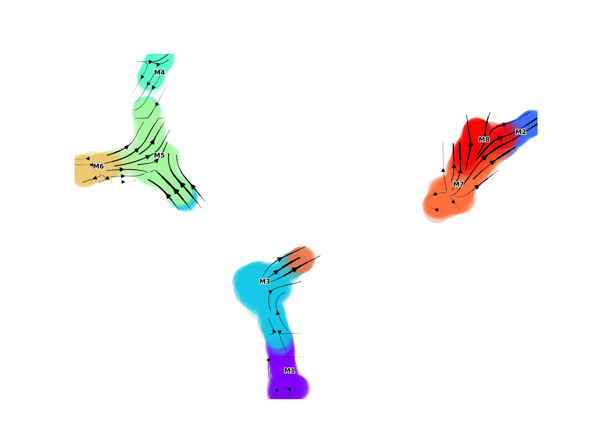
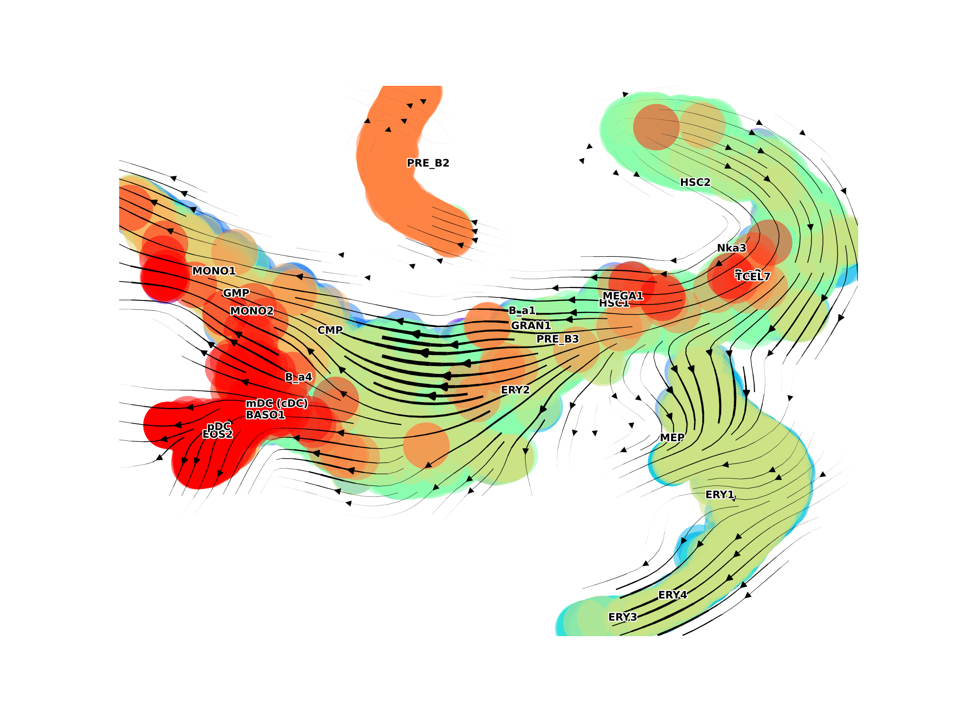
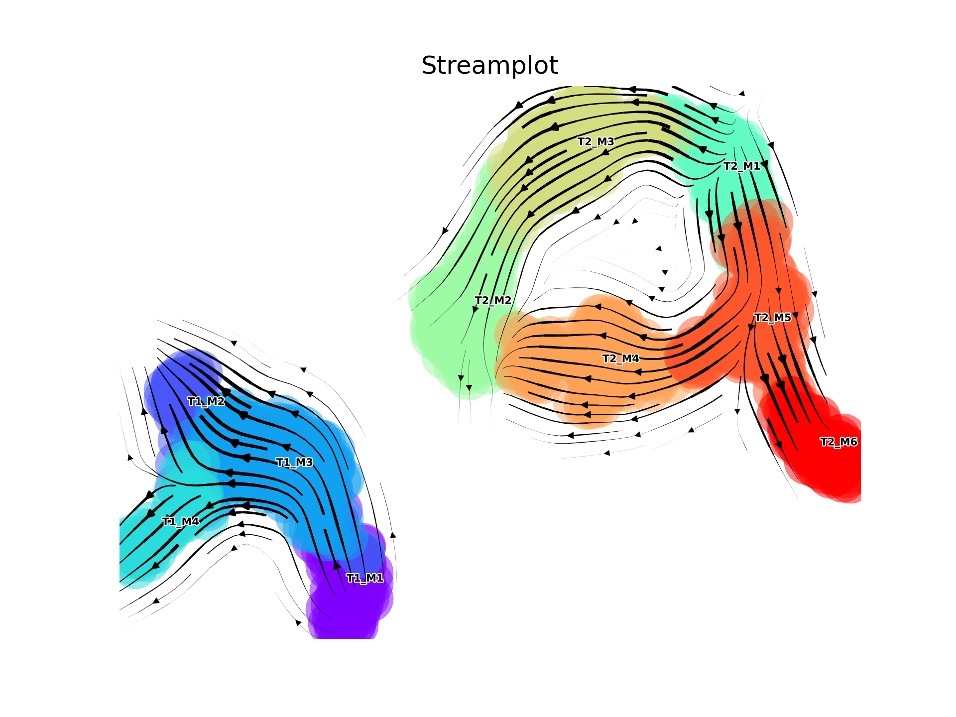
VIA.plotting_via.via_streamplot(via_object, embedding=None, density_grid=0.5, arrow_size=0.7, arrow_color='k', color_dict=None, arrow_style='-|>', max_length=4, linewidth=1, min_mass=1, cutoff_perc=5, scatter_size=500, scatter_alpha=0.5, marker_edgewidth=0.1, density_stream=2, smooth_transition=1, smooth_grid=0.5, color_scheme='annotation', add_outline_clusters=False, cluster_outline_edgewidth=0.001, gp_color='white', bg_color='black', dpi=300, title='Streamplot', b_bias=20, n_neighbors_velocity_grid=None, labels=None, use_sequentially_augmented=False, cmap='rainbow', show_text_labels=True)

Construct vector streamplot on the embedding to show a fine-grained view of inferred directions in the trajectory

Parameters:

• via_object –

• embedding (ndarray) – np.ndarray of shape (n_samples, 2) umap or other 2-d embedding on which to project the directionality of cells

• density_grid (float) –

• arrow_size (float) –

• arrow_color (str) –

• arrow_style –

• max_length (int) –

• linewidth (float) – width of lines in streamplot, default = 1

• min_mass –

• cutoff_perc (int) –

• scatter_size (int) – size of scatter points default =500

• scatter_alpha (float) – transpsarency of scatter points

• marker_edgewidth (float) – width of outline arround each scatter point, default = 0.1

• density_stream (int) –

• smooth_transition (int) –

• smooth_grid (float) –

• color_scheme (str) – str, default = ‘annotation’ corresponds to self.true_labels. Other options are ‘time’ (uses single-cell pseudotime) and ‘cluster’ (via cluster graph) and ‘other’. Alternatively provide labels as a list

• add_outline_clusters (bool) –

• cluster_outline_edgewidth –

• gp_color –

• bg_color –

• dpi –

• title –

• b_bias – default = 20. higher value makes the forward bias of pseudotime stronger

• n_neighbors_velocity_grid –

• labels (list) – list (will be used for the color scheme) or if a color_dict is provided these labels should match

• use_sequentially_augmented –

• cmap (str) –

Returns:

fig, ax

Datasets

VIA.datasets_via.cell_cycle(foldername='./')

Load cell cycle data as AnnData object

Args:

foldername (string): Directory of dataset

Returns:

AnnData object

VIA.datasets_via.cell_cycle_cyto_data(foldername='./')

Load cell cycle imagine based flow-cyto features AnnData object with n_obs × n_vars = 2036 × 38 obs: ‘cell_cycle_phase’ :param foldername (string) Default current directory. path to directory where you want to store the dataset

Returns:

anndata

VIA.datasets_via.embryoid_body(foldername='./')

Load embryoid body data as AnnData object

Args:

foldername (string): Directory to save dataset

Returns:

AnnData object

VIA.datasets_via.moffitt_preoptic(foldername='./')

Load preoptic hypothalamus mouse data from moffitt et al.,m as AnnData object

Args:

foldername (string): foldername (string): path to directory where you want to store the dataset ‘./’ current directory is default

Returns:

AnnData object

VIA.datasets_via.scATAC_hematopoiesis(foldername='./')

Load scATAC seq Hematopoiesis data as AnnData object

Args:

foldername (string): Directory of dataset

Returns:

AnnData object

VIA.datasets_via.scRNA_hematopoiesis(foldername='./')

Load scRNA seq Hematopoiesis data as AnnData object

Args:

foldername (string): Directory of dataset

Returns:

AnnData object

VIA.datasets_via.toy_disconnected(foldername='./')

Load Toy_Disconnected data as AnnData object

To access obs (label) as list, use AnnData.obs[‘group_id’].values.tolist()

Args:

foldername (string): Default current directory. path to directory where you want to store the dataset

Returns:

AnnData object

VIA.datasets_via.toy_multifurcating(foldername='./')

Load Toy_Multifurcating data as AnnData object

To access obs (label) as list, use AnnData.obs[‘group_id’].values.tolist()

Args:

foldername (string): foldername (string): path to directory where you want to store the dataset ‘./’ current directory is default

Returns:

AnnData object

VIA.datasets_via.zesta(foldername='./')

Returns: