5. Using time-series metadata (mESC Cytof)
In many developmental or longitudinal studies, the ages, experimental or developmental times are known. When such sampling point metadata are available, they can prove useful in guiding the graph construction and elucidating downstream analysis. The bottom of this tutorial shows what happens to the TI and visualization when you do not use the (time-series) sequential information to guide the analysis.
This example uses a mouse embryonic stem cell (mESC) differentiation time course collected with mass cytometry. This particularly example looks at the cells cultured in conditions favouring differentiation into the mesoderm lineage. Samples are collected over an 11 day period.
Load the data
The dataset consists of 89782 cells comprising ~ 7000 cells randomly sampled across each time point.
import scanpy as sc
import matplotlib.pyplot as plt
import pyVIA.core as via #from core_working import *
import pandas as pd
import numpy as np


data = pd.read_csv('/home/user/Trajectory/Datasets/mESC/mESC_7000perDay_noscaling_meso.csv')

marker_meso = ['Sca-1', 'CD41', 'Nestin', 'Desmin', 'CD24', 'FoxA2', 'Oct4', 'CD45', 'Ki67', 'Vimentin',
                     'Cdx2', 'Nanog', 'pStat3-705', 'Sox2', 'Flk-1', 'Tuj1', 'H3K9ac', 'Lin28', 'PDGFRa', 'EpCAM',
                     'CD44', 'GATA4', 'Klf4', 'CCR9', 'p53', 'SSEA1', 'bCatenin', 'IdU']
true_labels_numeric= data['day'].tolist()
print(f"Time series sampling points (days) {set(true_labels_numeric)}")
data = data[marker_meso] #using the subset of markers in the original paper

scale_arcsinh = 5 #commonly used arcsinh transformation for mass cytometry data
raw = data.values
raw = raw.astype('float')
raw = raw / scale_arcsinh
raw = np.arcsinh(raw)

adata = sc.AnnData(raw)
adata.var_names = data.columns
adata.obs['day_str'] = [str(i) for i in true_labels_numeric]
print(f"anndata shape {adata.shape}")
Time series sampling points (days) {0.0, 1.0, 2.0, 2.5, 3.0, 4.0, 5.0, 6.0, 7.0, 8.0, 9.0, 10.0, 11.0}
anndata shape (89782, 28)
Initialize and run VIA
You can play around with the graph-pruning parameters impacting the clustering granularity
edgepruning_clustering_resolution(float values between 0-1). larger values larger (but fewer) clustersthe cluster_graph_pruning(float values between 0-1) larger values retains more edges/connectivityroot(list) provide the cell index or a group-level label. We know that the initial state is at Day 0.0 so we allow Via to find the location of Day 0.0 cells that best fits an initial cluster. If using a group-level label, it must be an item found in true_label
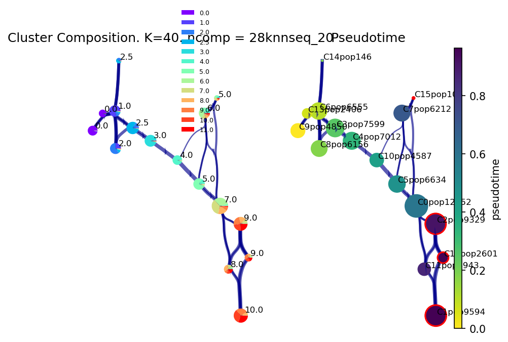
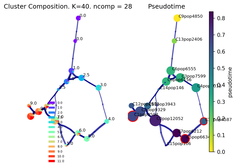
Plot the viagraph
Note that the clusters circled in red correspond to the identified (predicted) terminal fates and since we know the time-samples, we can see they correspond to cells in the final stages of development from Day 10-11.
f, ax1, ax2 = via.plot_piechart_viagraph(via_object=v0)
/home/user/anaconda3/envs/Via2Env_py10/lib/python3.10/site-packages/pyVIA/plotting_via.py:3092: UserWarning: No data for colormapping provided via 'c'. Parameters 'cmap' will be ignored
sct = ax.scatter(node_pos[:, 0], node_pos[:, 1],
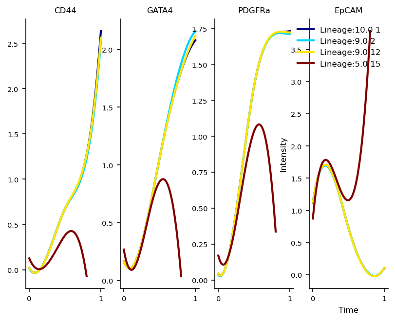
Protein Marker Dynamics
We expect the lineages associated with the differentiated mesoderm cells(Day 10/11 cells) to show an increase in Cd44, gata4 and pdgfra and a decrease in Epcam The Epcam high Lineage from Cluster 15 actually contains several day 9/10 cells
marker_genes = ['CD44', 'GATA4', 'PDGFRa', 'EpCAM']
df_genes = pd.DataFrame(adata[:, marker_genes].X)
df_genes.columns = marker_genes
f, axs= via.get_gene_expression(via_object=v0,gene_exp=df_genes, spline_order=3, n_splines=5)
plt.show()
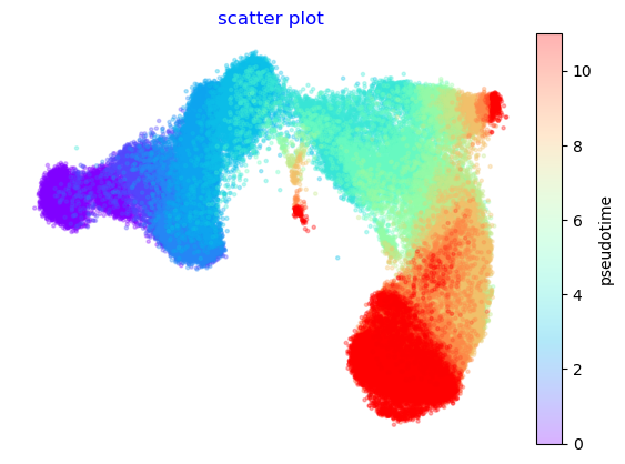
The Atlas Embedding
We use the knn-graph constructed in VIA which incorporates the sequential information in order to generate a 2D embedding of the data
atlas_embedding = via.via_atlas_emb(via_object=v0, min_dist=0.2, init_pos='via')
#via.run_atlas_emb(vi, graph=v0.csr_full_graph, n_components=2, spread=1.0, min_dist=0.3, init_pos='spectral', random_state=1, n_epochs=150))
X-input (89782, 28)
len membership and n_cells 89782 89782
n cell 89782
2023-10-10 15:03:03.170901 Computing embedding on sc-Viagraph
2023-10-10 15:03:03.235140 using via cluster graph to initialize embedding
f,ax=via.plot_scatter(embedding=atlas_embedding, labels= true_labels_numeric)
No artists with labels found to put in legend. Note that artists whose label start with an underscore are ignored when legend() is called with no argument.
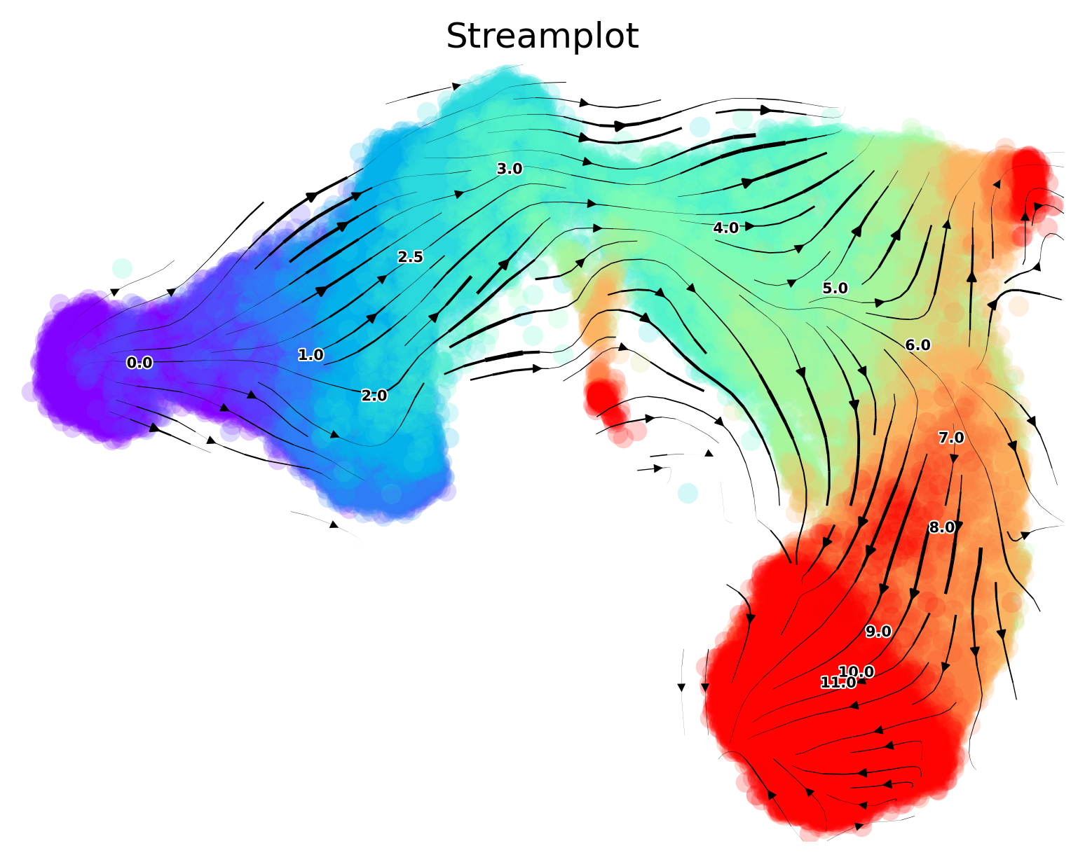
Streamplots for Cytof data
The cluster-level trajectory is projected onto the 2D embedding to visualize the more fine-grained progression
via.via_streamplot(v0, embedding=atlas_embedding, scatter_size=50, scatter_alpha=0.2, marker_edgewidth=0.01,
density_stream=1.5, density_grid=0.5, smooth_transition=1, smooth_grid=0.3)
plt.show()
/home/user/anaconda3/envs/Via2Env_py10/lib/python3.10/site-packages/scipy/sparse/_index.py:146: SparseEfficiencyWarning: Changing the sparsity structure of a csr_matrix is expensive. lil_matrix is more efficient.
self._set_arrayXarray(i, j, x)
/home/user/anaconda3/envs/Via2Env_py10/lib/python3.10/site-packages/pyVIA/core.py:1287: RuntimeWarning: divide by zero encountered in divide
T = T.multiply(csr_matrix(1.0 / np.abs(T).sum(1))) # rows sum to one
/home/user/anaconda3/envs/Via2Env_py10/lib/python3.10/site-packages/pyVIA/core.py:1318: RuntimeWarning: Mean of empty slice.
V_emb[i] = probs.dot(dX) - probs.mean() * dX.sum(0)
/home/user/anaconda3/envs/Via2Env_py10/lib/python3.10/site-packages/numpy/core/_methods.py:192: RuntimeWarning: invalid value encountered in scalar divide
ret = ret.dtype.type(ret / rcount)
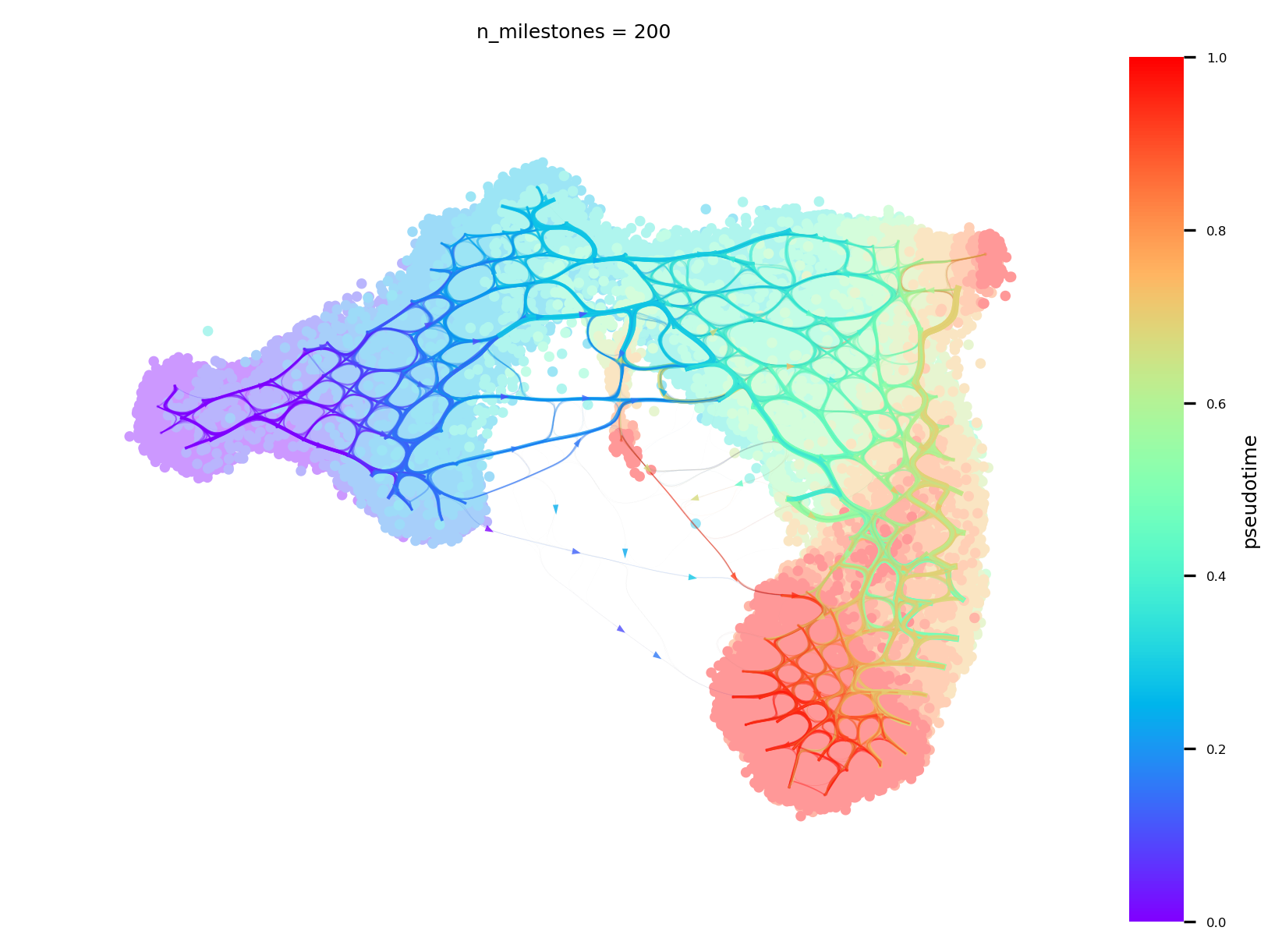
Draw The Atlas View with connectivities
A visualization unique to Via that combines the high-resolution edge and single-cell layouts
v0.embedding = atlas_embedding
f,ax=via.plot_atlas_view(via_object=v0,n_milestones=200, sc_labels_expression=true_labels_numeric, cmap='rainbow')
2023-10-10 15:14:30.048319 Computing Edges
2023-10-10 15:14:30.048365 Start finding milestones
2023-10-10 15:14:47.168789 End milestones with 200
2023-10-10 15:14:48.656038 Recompute weights
2023-10-10 15:14:48.713622 pruning milestone graph based on recomputed weights
2023-10-10 15:14:48.715549 Graph has 1 connected components before pruning
2023-10-10 15:14:48.716435 Graph has 1 connected components after pruning
2023-10-10 15:14:48.716688 Graph has 1 connected components after reconnecting
2023-10-10 15:14:48.719559 regenerate igraph on pruned edges
2023-10-10 15:14:48.766860 Setting numeric label as time_series_labels or other sequential metadata for coloring edges
2023-10-10 15:14:49.010023 Making smooth edges
inside add sc embedding second if
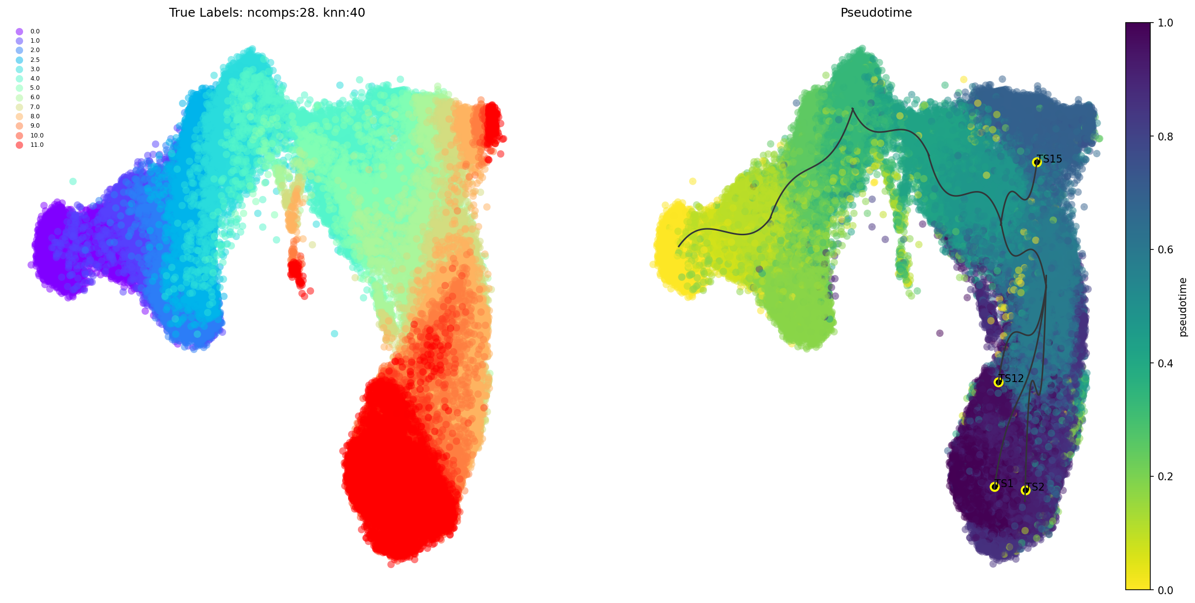
Terminal states and pathways
The high-level direction from root to different final states is shown here. The final states are marked in yellow
via.plot_trajectory_curves(via_object=v0, draw_all_curves=False) #Setting 'draw_all_curves' to False helps highlight major pathways
plt.show()
100% (11 of 11) |########################| Elapsed Time: 0:00:00 Time: 0:00:00
100% (11 of 11) |########################| Elapsed Time: 0:00:00 Time: 0:00:00
100% (11 of 11) |########################| Elapsed Time: 0:00:00 Time: 0:00:00
100% (11 of 11) |########################| Elapsed Time: 0:00:00 Time: 0:00:00
100% (11 of 11) |########################| Elapsed Time: 0:00:00 Time: 0:00:00
100% (11 of 11) |########################| Elapsed Time: 0:00:00 Time: 0:00:00
100% (11 of 11) |########################| Elapsed Time: 0:00:00 Time: 0:00:00
100% (11 of 11) |########################| Elapsed Time: 0:00:00 Time: 0:00:00
100% (11 of 11) |########################| Elapsed Time: 0:00:00 Time: 0:00:00
2023-10-10 15:19:22.164658 Super cluster 1 is a super terminal with sub_terminal cluster 1
2023-10-10 15:19:22.166815 Super cluster 2 is a super terminal with sub_terminal cluster 2
2023-10-10 15:19:22.166871 Super cluster 12 is a super terminal with sub_terminal cluster 12
2023-10-10 15:19:22.166903 Super cluster 15 is a super terminal with sub_terminal cluster 15
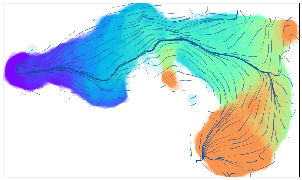
Animated Trajectory
Fine grained vector fields in action
via.animate_streamplot(v0, embedding=atlas_embedding,saveto='/home/user/Trajectory/Datasets/mESC/mesc_timeseries_stream_animation_oct2023.gif') #saveto='.../filename.gif')
/home/user/anaconda3/envs/Via2Env_py10/lib/python3.10/site-packages/pyVIA/core.py:1318: RuntimeWarning: Mean of empty slice.
V_emb[i] = probs.dot(dX) - probs.mean() * dX.sum(0)
/home/user/anaconda3/envs/Via2Env_py10/lib/python3.10/site-packages/numpy/core/_methods.py:192: RuntimeWarning: invalid value encountered in scalar divide
ret = ret.dtype.type(ret / rcount)
2023-10-10 15:50:11.443156 Inside animated. File will be saved to location /home/user/Trajectory/Datasets/mESC/mesc_timeseries_stream_animation_oct2023.gif
total number of stream lines 410
0%| | 0/250 [00:00<?, ?it/s]
MovieWriter imagemagick unavailable; using Pillow instead.
(<Figure size 1000x600 with 1 Axes>, <Axes: >)
from IPython.display import Image
with open('/home/user/Trajectory/Datasets/mESC/mesc_timeseries_stream_animation_oct2023.gif','rb') as file:
display(Image(file.read()))
Not using time-series data to guide the analysis
When choosing not to use the available experimental time-stamps, we see that the overall Trajectory is more difficult to interpret and chronology is less clear (as seen when plotting the viagraph below)
knn=40
cluster_graph_pruning = 0.15
edgepruning_clustering_resolution=0.3
random_seed = 0
root = [0.0] #since the root corresponds to a group level initial state we set dataset = 'group'
v_notime = via.VIA(adata.X, true_label=true_labels_numeric, edgepruning_clustering_resolution=edgepruning_clustering_resolution, edgepruning_clustering_resolution_local=1, knn=knn,
cluster_graph_pruning=cluster_graph_pruning, piegraph_arrow_head_width=0.6,
too_big_factor=0.3, resolution_parameter=1,
root_user=root, dataset='group', random_seed=random_seed,
is_coarse=True, preserve_disconnected=False, pseudotime_threshold_TS=40, x_lazy=0.99,
alpha_teleport=0.99)
v_notime.run_VIA()
2023-10-10 17:22:51.827898 Running VIA over input data of 89782 (samples) x 28 (features)
2023-10-10 17:22:51.827943 Knngraph has 40 neighbors
2023-10-10 17:23:32.546462 Finished global pruning of 40-knn graph used for clustering at level of 0.3. Kept 55.2 % of edges.
2023-10-10 17:23:33.360124 Number of connected components used for clustergraph is 1
2023-10-10 17:23:42.945437 Commencing community detection
2023-10-10 17:23:48.961073 Finished running Leiden algorithm. Found 24 clusters.
2023-10-10 17:23:49.031375 Merging 8 very small clusters (<10)
2023-10-10 17:23:49.047839 Finished detecting communities. Found 16 communities
2023-10-10 17:23:49.053183 Making cluster graph. Global cluster graph pruning level: 0.15
2023-10-10 17:23:49.514431 Graph has 1 connected components before pruning
2023-10-10 17:23:49.520669 Graph has 1 connected components after pruning
2023-10-10 17:23:49.521053 Graph has 1 connected components after reconnecting
2023-10-10 17:23:49.521919 0.0% links trimmed from local pruning relative to start
2023-10-10 17:23:49.521948 69.8% links trimmed from global pruning relative to start
2023-10-10 17:23:49.543246 component number 0 out of [0]
2023-10-10 17:23:49.637670 group root method
2023-10-10 17:23:49.637712 for component 0, the root is 0.0 and ri 0.0
cluster 0 has majority 7.0
cluster 1 has majority 10.0
2023-10-10 17:23:49.858094 New root is 1 and majority 10.0
cluster 2 has majority 9.0
cluster 3 has majority 2.5
cluster 4 has majority 3.0
cluster 5 has majority 5.0
cluster 6 has majority 1.0
cluster 7 has majority 6.0
cluster 8 has majority 2.0
cluster 9 has majority 0.0
2023-10-10 17:23:49.934760 New root is 9 and majority 0.0
cluster 10 has majority 4.0
cluster 11 has majority 8.0
cluster 12 has majority 9.0
cluster 13 has majority 0.0
cluster 14 has majority 2.5
cluster 15 has majority 5.0
2023-10-10 17:23:49.978782 Computing lazy-teleporting expected hitting times
2023-10-10 17:23:50.514672 ended all multiprocesses, will retrieve and reshape
try rw2 hitting times setup
start computing walks with rw2 method
g.indptr.size, 17
/home/user/anaconda3/envs/Via2Env_py10/lib/python3.10/site-packages/pecanpy/graph.py:90: UserWarning: WARNING: Implicitly set node IDs to the canonical node ordering due to missing IDs field in the raw CSR npz file. This warning message can be suppressed by setting implicit_ids to True in the read_npz function call, or by setting the --implicit_ids flag in the CLI
  warnings.warn(
memory for rw2 hittings times 2. Using rw2 based pt
do scaling of pt
2023-10-10 17:23:54.358993 Identifying terminal clusters corresponding to unique lineages...
2023-10-10 17:23:54.359042 Closeness:[1, 4, 5, 9, 10, 13]
2023-10-10 17:23:54.359053 Betweenness:[1, 4, 5, 7, 8, 9, 10, 13]
2023-10-10 17:23:54.359059 Out Degree:[1, 2, 4, 5, 9, 10, 12, 13, 15]
2023-10-10 17:23:54.359431 Terminal clusters corresponding to unique lineages in this component are [1, 10, 5]
TESTING rw2_lineage probability at memory 5
testing rw2 lineage probability at memory 5
g.indptr.size, 17
/home/user/anaconda3/envs/Via2Env_py10/lib/python3.10/site-packages/pecanpy/graph.py:90: UserWarning: WARNING: Implicitly set node IDs to the canonical node ordering due to missing IDs field in the raw CSR npz file. This warning message can be suppressed by setting implicit_ids to True in the read_npz function call, or by setting the --implicit_ids flag in the CLI
  warnings.warn(
2023-10-10 17:23:57.703638 Cluster or terminal cell fate 1 is reached 223.0 times
2023-10-10 17:23:57.741600 Cluster or terminal cell fate 10 is reached 606.0 times
2023-10-10 17:23:57.770042 Cluster or terminal cell fate 5 is reached 997.0 times
2023-10-10 17:23:57.790720 There are (3) terminal clusters corresponding to unique lineages {1: 10.0, 10: 4.0, 5: 5.0}
2023-10-10 17:23:57.790771 Begin projection of pseudotime and lineage likelihood
2023-10-10 17:24:02.856437 Cluster graph layout based on forward biasing
2023-10-10 17:24:02.857501 Starting make edgebundle viagraph...
2023-10-10 17:24:02.857518 Make via clustergraph edgebundle
2023-10-10 17:24:03.108995 Hammer dims: Nodes shape: (16, 2) Edges shape: (70, 3)
2023-10-10 17:24:03.112835 Graph has 1 connected components before pruning
2023-10-10 17:24:03.118067 Graph has 7 connected components after pruning
2023-10-10 17:24:03.129269 Graph has 1 connected components after reconnecting
2023-10-10 17:24:03.129927 55.7% links trimmed from local pruning relative to start
2023-10-10 17:24:03.129956 72.9% links trimmed from global pruning relative to start
2023-10-10 17:24:03.215031 Time elapsed 56.7 seconds
/home/user/anaconda3/envs/Via2Env_py10/lib/python3.10/site-packages/scipy/sparse/_index.py:103: SparseEfficiencyWarning: Changing the sparsity structure of a csr_matrix is expensive. lil_matrix is more efficient.
  self._set_intXint(row, col, x.flat[0])
f, ax1, ax2 = via.plot_piechart_viagraph(via_object=v_notime)
/home/user/anaconda3/envs/Via2Env_py10/lib/python3.10/site-packages/pyVIA/plotting_via.py:3092: UserWarning: No data for colormapping provided via 'c'. Parameters 'cmap' will be ignored
  sct = ax.scatter(node_pos[:, 0], node_pos[:, 1],
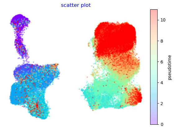
Using UMAP instead of Via’s cartographic embeddings
As shown below, if once uses UMAP instead of the TI adjusted embedding from Via, then the early and late stages are disconnected
import umap
embedding_umap = umap.UMAP(random_state=42, n_neighbors=15, init='spectral', min_dist=0.2).fit_transform(adata.X)
f,ax=via.plot_scatter(embedding=embedding_umap, labels=true_labels_numeric)
No artists with labels found to put in legend. Note that artists whose label start with an underscore are ignored when legend() is called with no argument.