Stavia Spatially aware cartography on MERFISH
This tutorial focuses on how to perform TI analysis on MERFISH (Moffitt 2018), a spatial gene expression profile of preoptic mouse hypothalamus. We are able to integrate the single-cell spatial contexts and their gene expressions to present a cartographic view of the system and the relationships between cell populations.
Import Libraries
import scanpy as sc
import pandas as pd
import squidpy as sq
import matplotlib.pyplot as plt
import pyVIA.core as via
import numpy as np
sc.logging.print_header()
from datetime import datetime
from collections import defaultdict
import matplotlib.cm as cm
from pyVIA import datasets_via as datasets
import warnings
warnings.filterwarnings("ignore")
C:\Users\Kevin tsia\anaconda3\envs\via2\Lib\site-packages\phate\__init__.py
scanpy==1.9.8 anndata==0.10.5.post1 umap==0.5.5 numpy==1.26.4 scipy==1.12.0 pandas==2.2.1 scikit-learn==1.4.1.post1 statsmodels==0.14.1 igraph==0.11.4 pynndescent==0.5.11
Load Dataset
Load the dataset and select a z plane to get a 2D tissue section to work on.
# load the pre-processed dataset
# adata = sq.datasets.merfish() #AnnData object with n_obs × n_vars = 73655 × 161

# Download data (can also copy this file from Via Github Datasets folder)
adata = datasets.moffitt_preoptic()
print(adata)
'''
AnnData object with n_obs × n_vars = 73655 × 161
    obs: 'Cell_ID', 'Animal_ID', 'Animal_sex', 'Behavior', 'Bregma', 'Centroid_X', 'Centroid_Y', 'Cell_class', 'Neuron_cluster_ID', 'batch'
    uns: 'Cell_class_colors'
    obsm: 'spatial', 'spatial3d'
    animal id {1}
animal sex {'Female'}
animal behaviour {'Naive'}
Bregma {1.0, -28.999999999999996, 6.0, -24.0, 11.0, -19.0, 16.0, -14.000000000000002, 21.0, -9.0, 26.0, -4.0}
161
'''
# selecting a slice at Bregma -29 and subsetting the anndata
bregma =-28.999999999999996

adata = adata[adata.obs.Bregma == bregma]  # View of AnnData object with n_obs × n_vars = 6185 × 161 #26
AnnData object with n_obs × n_vars = 73655 × 161
    obs: 'Cell_ID', 'Animal_ID', 'Animal_sex', 'Behavior', 'Bregma', 'Centroid_X', 'Centroid_Y', 'Cell_class', 'Neuron_cluster_ID', 'batch'
    uns: 'Cell_class_colors'
    obsm: 'spatial', 'spatial3d'
Cell annotations
Organise cell annotations for validation purpose in later sections.
# do some preliminary house-keeping of labels (this is optional and we do it here because we want to have better automatic color separation between cell types that have similar starting letters)
true_label = [i if i != 'Excitatory' else 'xExcitatory' for i in adata.obs['Cell_class']] #relabeling Excitatory to more easily distinguish colors between Endothelial and Excitatory
cell_class_labels = [i for i in adata.obs['Cell_class']]
# simplifying class labels for easier color coding/visualization
for ei, i in enumerate(cell_class_labels):
    if i in ['OD Immature 2', 'OD Immature 1']: true_label[ei] = 'OD_Immature'
    if i in ['OD Mature 1', 'OD Mature 2','OD Mature 3','OD Mature 4']: true_label[ei] = 'OD_Mature'
    if i in ['Endothelial 1','Endothelial 2','Endothelial 3']: true_label[ei] = 'Endothelial'

adata.obs['true_label'] = [i for i in true_label]
set_true_label = list(set(true_label))
Tissue section scatter plot colored based on cell types
#optionally create a celltype_to_color dictionary so that cell types are consistenly plotted with the same colors in all plots
color_dict = {}
set_labels = list(set(true_label))
set_labels.sort(reverse=False)#True)
palette = cm.get_cmap('rainbow', len(set_labels))
cmap_ = palette(range(len(set_labels)))
for index, value in enumerate(set_labels):
color_dict[value] = cmap_[index]
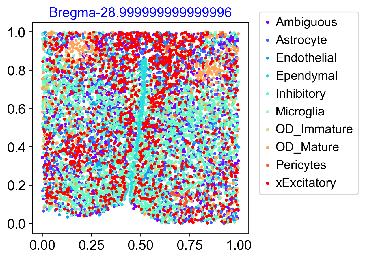
# have a look at the major cell types on the tissue slice
coords = adata.obsm['spatial']
f, ax = via.plot_scatter(adata.obsm['spatial'], labels=true_label, color_dict=color_dict, show_legend=True, cmap='rainbow', alpha=1, s=10, title='Bregma'+str(bregma), text_labels=False, hide_axes_ticks=False)
ax.legend(bbox_to_anchor=(1.05, 1.05), borderaxespad=0)
plt.show()
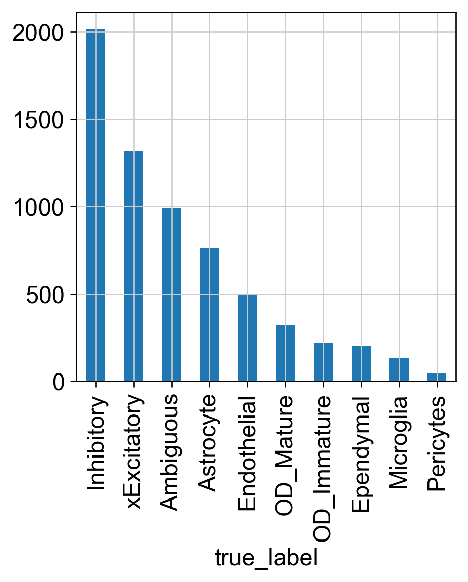
Cell Population
# Cell population in each major celltype
d = {val: true_label.count(val) for val in set(adata.obs['true_label'])}
display(d)
ax = adata.obs['true_label'].value_counts().plot.bar()
{'OD_Mature': 323,
 'OD_Immature': 221,
 'Astrocyte': 763,
 'Endothelial': 495,
 'Ambiguous': 992,
 'xExcitatory': 1319,
 'Inhibitory': 2013,
 'Pericytes': 46,
 'Ependymal': 202,
 'Microglia': 135}
Run StaVia
There are 2 main steps in how we can incorporate spatial information. Step 1: Modifying the gene-expression such that we smooth a cell’s gene expression with that of its spatial neighbors. Step 2: uses spatial information in the Trajectory inference computation.
Keep do_spatial = True if you would like to incorporate spatial data to the VIA analysis.
Step 1 Parameters:
We can adjust the weight of influence of the spatial data for by tuning the parameters:
spatial_knn: number of knn based on spatial-cell-location.
spatial_weight: the weight given to gene-expression of spatial neighbors when recomputing gene-expression to include expression of neighbors on tissue slice
spatial_knn_input = 6
spatial_weight = 0.3
Step 2 Parameters:
do_spatial_knn=True. #True means that spatial information is used to adjust the predicted trajectory
do_spatial_layout= True/False. #True means that the spatial information is used to modify the graph-layout, but should only be used when all cells come from the same tissue.
spatial_coords = coords. #ndarray (ncells x 2) of cell location on tissue slice(s)
spatial_knn_trajectory =6. #is the number of spatial neighbors used in the gene-spatial knn graph. this is different from 'knn' parameter which selects neighbors based on gene/feature input distances
If you have previously run VIA or other clustering algorithms, we can provide the clustering prelabels to initialise the VIA run.
In the above senario, we can set do_rank_genes = True to get clustering based DEGs among different cell types. This step can be carried out after the VIA run with the computed clustering labels.
# setting parameters for StaVia
cluster_graph_pruning = 0.5 # (0-1) higher value means more edges in the StaVia TI-clustergraph are retained
edgepruning_clustering_resolution = 0.3 #(0-1) # higher values means bigger and fewer clusters
random_seed = 2
knn =10 # 10, 20, 30 are good as well
neighboring_terminal_states_threshold = 4
root = ["Ependymal"]

do_spatial =True
n_pcs =50

import random
pseudorand = random.randint(0, 1000)
#SPATIAL STEP 1 (modify gene expression of input data based on expression of spatial neighbors). This is computed before run_via() and is optional
if do_spatial:
    coords=adata.obsm['spatial']

    spatial_knn_input = 6 # higher values of spatial_knn results in more gene-smoothing across neighboring cells on the slice
    spatial_weight = 0.3
    X_spatial_exp = via.spatial_input(X_genes = adata.X, spatial_coords=coords, knn_spatial=spatial_knn_input, spatial_weight=spatial_weight)

    adata.obsm['X_spatial_adjusted'] = X_spatial_exp
    adata.obsm["spatial_pca"] = sc.tl.pca(adata.obsm['X_spatial_adjusted'],n_comps=n_pcs)

    input = adata.obsm['spatial_pca'][:,0:n_pcs]
    print(f'end X_spatial input')
else:
    spatial_knn_input = 0
    spatial_knn_trajectory = 0
    coords = None
    spatial_weight = 0
    sc.tl.pca(adata, n_comps=n_pcs)
    input = adata.obsm['X_pca'][:,0:n_pcs]


WORK_PATH = './'
use_prelabels = False #True
if use_prelabels:
    #if you have saved a set of cluster labels (from a previous run of StaVia or another clustering method) then you can use them
    pre_labels =  pd.read_csv(WORK_PATH + '/Viagraphs/bregma_m28p9/spatialknn6/PARC_Bregma-28_pseudrand320.csv')
    pre_labels = pre_labels['parc'].tolist()
    print('using prelabels',set(pre_labels))

    adata.obs['parc'] = ['c' + str(i) for i in pre_labels]
    adata.obs['parc_num'] = [i for i in pre_labels]

else: pre_labels = None

# SPATIAL STEP 2 (Via graph spatial parameters)
# set: do_spatial_knn=do_spatial, do_spatial_layout= do_spatial, spatial_coords = coords, spatial_knn=spatial_knn_trajectory (can be the same value as spatial_knn_input or can be tuned)
# spatial_coords, ndarray (ncells x 2) of cell location on tissue slice(s)
# do_spatial_layout = True means that the spatial information is used to modify the graph-layout, but should only be used when all cells come from the same tissue.
# spatial_knn (int) is the number of spatial neighbors used in the gene-spatial knn graph. this is different from 'knn' parameter which selects neighbors based on gene/feature input distances
spatial_knn_trajectory = 6 # e.g. set it to the same value as spatial_knn_input, but the user can change this
v0 = via.VIA(data=input, true_label=true_label, edgepruning_clustering_resolution=edgepruning_clustering_resolution, labels=pre_labels,
                 edgepruning_clustering_resolution_local=1, knn=knn,
                 cluster_graph_pruning=cluster_graph_pruning,
                 neighboring_terminal_states_threshold=neighboring_terminal_states_threshold,
                 too_big_factor=0.3, resolution_parameter=1,
                 root_user=root, dataset='group', random_seed=random_seed,
                 is_coarse=True, preserve_disconnected=True, pseudotime_threshold_TS=40, x_lazy=0.99,
                 alpha_teleport=0.99, edgebundle_pruning=cluster_graph_pruning, edgebundle_pruning_twice=True, do_spatial_knn=do_spatial, do_spatial_layout= do_spatial, spatial_coords = coords, spatial_knn=spatial_knn_trajectory)
v0.run_VIA()
2024-03-01 17:14:57.121364	These slices are present: ['slice1']
x_coords shape (6509, 2)
x_genes shape (6509, 161)
nsamples (slices) 6509
2024-03-01 17:14:58.152594	Shape spatial neighbors and data shape (6509, 6) (6509, 6)
2024-03-01 17:14:58.199468	Spatial gene smoothing... (6509, 6)
end X_spatial input
2024-03-01 17:14:58.426018	Running VIA over input data of 6509 (samples) x 50 (features)
2024-03-01 17:14:58.426018	Knngraph has 10 neighbors
2024-03-01 17:15:00.582737	Since no slice-labels were provided, all cells are assumed to be from the same tissue slice
2024-03-01 17:15:00.582737	Using spatial information to guide knn graph construction. Note! If cells are from different slices of tissue, provide a list of tissue-slice IDs
2024-03-01 17:15:00.598338	These slices are present: ['slice1']
2024-03-01 17:15:01.614877	Shape neighbors (6509, 10) and spatial neighbors (6509, 6)
2024-03-01 17:15:01.614877	Shape of spatially augmented neighbors (6509, 16)
2024-03-01 17:15:01.790113	Finished global pruning of 10-knn graph used for clustering at level of 0.3. Kept 54.2 % of edges.
2024-03-01 17:15:01.790113	using spatial coords to augment clustergraph
2024-03-01 17:15:01.805736	Number of connected components used for clustergraph  is 1
2024-03-01 17:15:01.925219	Commencing community detection
2024-03-01 17:15:01.994793	Finished community detection. Found 268 clusters.
2024-03-01 17:15:01.994793	Merging 224 very small clusters (<10)
2024-03-01 17:15:01.994793	Finished detecting communities. Found 44 communities
2024-03-01 17:15:01.994793	Making cluster graph. Global cluster graph pruning level: 0.5
2024-03-01 17:15:02.010419	Graph has 1 connected components before pruning
2024-03-01 17:15:02.010419	Graph has 1 connected components after pruning
2024-03-01 17:15:02.010419	Graph has 1 connected components after reconnecting
2024-03-01 17:15:02.010419	23.8% links trimmed from local pruning relative to start
2024-03-01 17:15:02.026042	component number 0 out of  [0]
2024-03-01 17:15:02.026042	group root method
2024-03-01 17:15:02.026042	for component 0, the root is Ependymal and ri Ependymal
cluster 0 has majority Endothelial
cluster 1 has majority Astrocyte
cluster 2 has majority Astrocyte
cluster 3 has majority xExcitatory
cluster 4 has majority xExcitatory
cluster 5 has majority Inhibitory
cluster 6 has majority Ambiguous
cluster 7 has majority OD_Mature
cluster 8 has majority Inhibitory
cluster 9 has majority Ependymal
2024-03-01 17:15:02.057288	New root is 9 and majority Ependymal
cluster 10 has majority Inhibitory
cluster 11 has majority OD_Immature
cluster 12 has majority Inhibitory
cluster 13 has majority Astrocyte
cluster 14 has majority xExcitatory
cluster 15 has majority Ambiguous
cluster 16 has majority Inhibitory
cluster 17 has majority Inhibitory
cluster 18 has majority Inhibitory
cluster 19 has majority Inhibitory
cluster 20 has majority xExcitatory
cluster 21 has majority Microglia
cluster 22 has majority xExcitatory
cluster 23 has majority xExcitatory
cluster 24 has majority Ambiguous
cluster 25 has majority Inhibitory
cluster 26 has majority Endothelial
cluster 27 has majority OD_Immature
cluster 28 has majority Inhibitory
cluster 29 has majority Pericytes
cluster 30 has majority OD_Mature
cluster 31 has majority Inhibitory
cluster 32 has majority xExcitatory
cluster 33 has majority Inhibitory
cluster 34 has majority xExcitatory
cluster 35 has majority Inhibitory
cluster 36 has majority Inhibitory
cluster 37 has majority xExcitatory
cluster 38 has majority Inhibitory
cluster 39 has majority Inhibitory
cluster 40 has majority xExcitatory
cluster 41 has majority Inhibitory
cluster 42 has majority xExcitatory
cluster 43 has majority xExcitatory
2024-03-01 17:15:02.057288	Computing lazy-teleporting expected hitting times
2024-03-01 17:15:12.960702	Ended all multiprocesses, will retrieve and reshape
2024-03-01 17:15:12.991944	start computing walks with rw2 method
memory for rw2 hittings times  2. Using rw2 based pt
2024-03-01 17:15:19.629476	Identifying terminal clusters corresponding to unique lineages...
2024-03-01 17:15:19.629476	Closeness:[0, 3, 5, 6, 7, 11, 15, 16, 17, 20, 21, 24, 27, 29, 30, 34, 43]
2024-03-01 17:15:19.629476	Betweenness:[0, 1, 2, 3, 4, 6, 7, 9, 11, 12, 13, 16, 17, 20, 21, 24, 26, 27, 29, 30, 33, 34, 36, 37, 39, 40, 42, 43]
2024-03-01 17:15:19.629476	Out Degree:[0, 3, 5, 6, 7, 9, 11, 15, 16, 20, 21, 24, 26, 27, 28, 29, 30, 33, 34, 35, 36, 37, 38, 40, 41, 43]
2024-03-01 17:15:19.629476	Cluster 0 had 4 or more neighboring terminal states [3, 5, 6, 7, 11, 15, 16, 20, 21, 24, 26, 27, 29, 30, 34, 36, 37, 43] and so we removed cluster 37
2024-03-01 17:15:19.629476	Cluster 3 had 4 or more neighboring terminal states [0, 7, 11, 21, 24, 26, 27] and so we removed cluster 3
2024-03-01 17:15:19.629476	Cluster 5 had 4 or more neighboring terminal states [0, 6, 7, 11, 15, 16, 20, 24, 26, 29, 40] and so we removed cluster 20
2024-03-01 17:15:19.629476	Cluster 6 had 4 or more neighboring terminal states [0, 5, 11, 15, 16, 21, 26, 27, 29, 36, 40] and so we removed cluster 36
2024-03-01 17:15:19.629476	Cluster 7 had 4 or more neighboring terminal states [0, 5, 11, 15, 16, 21, 24, 27, 30, 34, 43] and so we removed cluster 21
2024-03-01 17:15:19.629476	Cluster 11 had 4 or more neighboring terminal states [0, 5, 6, 7, 15, 16, 24, 27, 34, 40, 43] and so we removed cluster 27
2024-03-01 17:15:19.629476	Cluster 15 had 4 or more neighboring terminal states [0, 5, 6, 7, 11, 16, 24, 26, 29, 40, 43] and so we removed cluster 26
2024-03-01 17:15:19.629476	Cluster 16 had 4 or more neighboring terminal states [0, 5, 6, 7, 11, 15, 24] and so we removed cluster 6
2024-03-01 17:15:19.629476	Cluster 24 had 4 or more neighboring terminal states [0, 5, 7, 11, 15, 16, 30, 34, 43] and so we removed cluster 34
2024-03-01 17:15:19.629476	Cluster 43 had 4 or more neighboring terminal states [0, 7, 11, 15, 24] and so we removed cluster 11
2024-03-01 17:15:19.629476	Terminal clusters corresponding to unique lineages in this component are [0, 5, 7, 15, 16, 24, 29, 30, 40, 43]
2024-03-01 17:15:19.629476	Calculating lineage probability at memory 5
2024-03-01 17:15:24.265260	Cluster or terminal cell fate 0 is reached 1000.0 times
2024-03-01 17:15:24.327753	Cluster or terminal cell fate 5 is reached 601.0 times
2024-03-01 17:15:24.374627	Cluster or terminal cell fate 7 is reached 1000.0 times
2024-03-01 17:15:24.421496	Cluster or terminal cell fate 15 is reached 999.0 times
2024-03-01 17:15:24.492464	Cluster or terminal cell fate 16 is reached 467.0 times
2024-03-01 17:15:24.535213	Cluster or terminal cell fate 24 is reached 790.0 times
2024-03-01 17:15:24.597706	Cluster or terminal cell fate 29 is reached 904.0 times
2024-03-01 17:15:24.644578	Cluster or terminal cell fate 30 is reached 998.0 times
2024-03-01 17:15:24.726092	Cluster or terminal cell fate 40 is reached 99.0 times
2024-03-01 17:15:24.753152	Cluster or terminal cell fate 43 is reached 1000.0 times
2024-03-01 17:15:24.784401	There are (10) terminal clusters corresponding to unique lineages {0: 'Endothelial', 5: 'Inhibitory', 7: 'OD_Mature', 15: 'Ambiguous', 16: 'Inhibitory', 24: 'Ambiguous', 29: 'Pericytes', 30: 'OD_Mature', 40: 'xExcitatory', 43: 'xExcitatory'}
2024-03-01 17:15:24.784401	Begin projection of pseudotime and lineage likelihood
2024-03-01 17:15:25.890315	Cluster graph layout based on forward biasing
2024-03-01 17:15:25.890315	Graph has 1 connected components before pruning
2024-03-01 17:15:25.890315	Graph has 14 connected components after pruning
2024-03-01 17:15:25.905938	Graph has 1 connected components after reconnecting
2024-03-01 17:15:25.905938	90.2% links trimmed from local pruning relative to start
2024-03-01 17:15:25.905938	92.7% links trimmed from global pruning relative to start
2024-03-01 17:15:25.905938	Additional Visual cluster graph pruning for edge bundling at level: 0.15
2024-03-01 17:15:25.905938	Make via clustergraph edgebundle
2024-03-01 17:15:28.811682	Hammer dims: Nodes shape: (44, 2) Edges shape: (914, 3)
2024-03-01 17:15:28.827307	Time elapsed 29.2 seconds
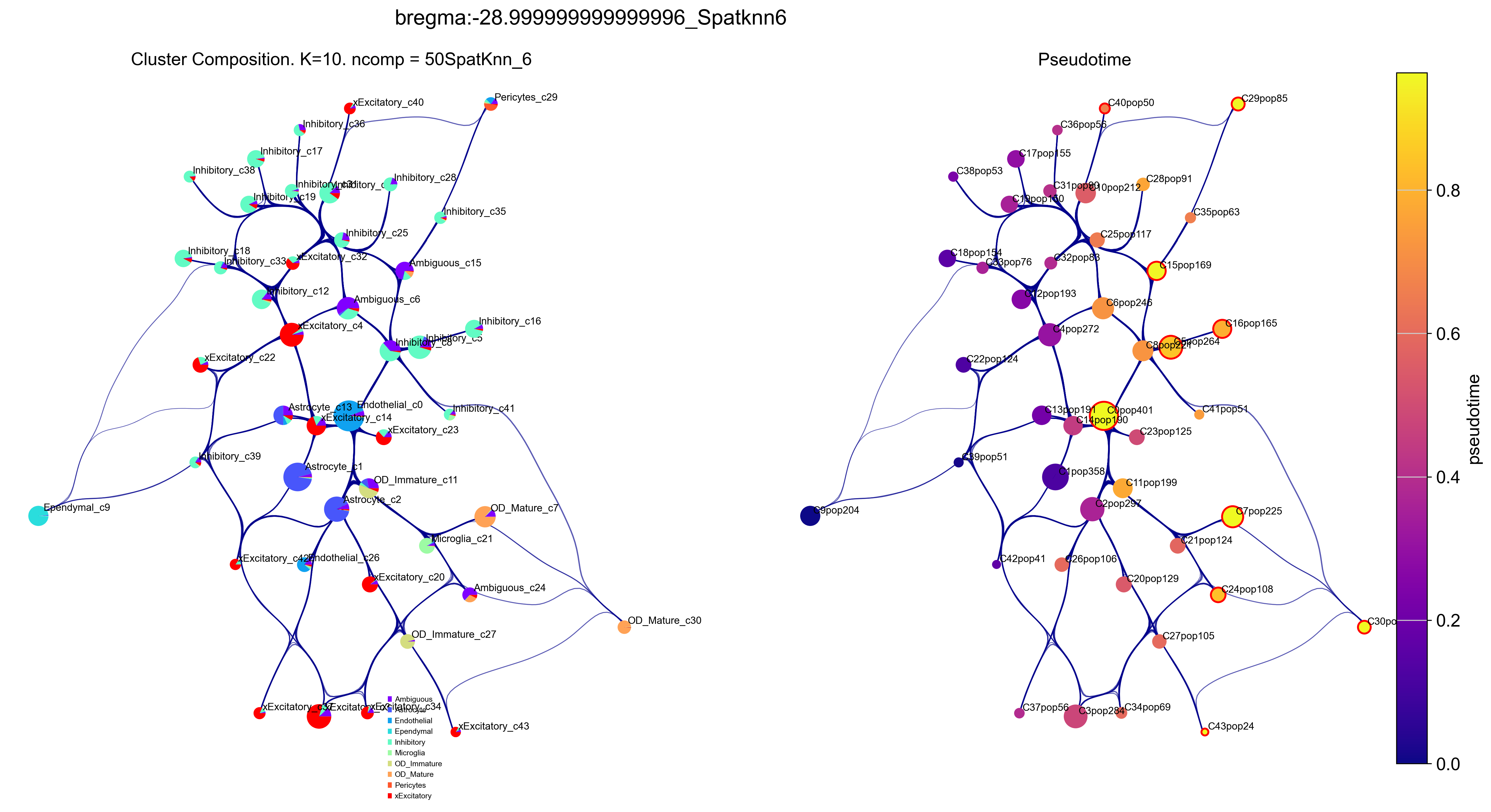
Right plot is VIA graph with cell type label and visualised cell type population in each clusters.
Left plot is colored by pseudo time with a ‘rainbow’ colormap.
f2, ax1, ax2 = via.plot_piechart_viagraph(via_object=v0, cmap_piechart='rainbow', cmap='plasma', pie_size_scale=0.4, linewidth_edge=0.6,
                                          reference_labels=true_label, headwidth_arrow=0.001,
                                          highlight_terminal_clusters=True, show_legend=True)
f2.set_size_inches(20,10)
f2.suptitle('bregma:'+str(bregma)+'_Spatknn'+str(spatial_knn_trajectory))
plt.show()
Via graph visualization tuning
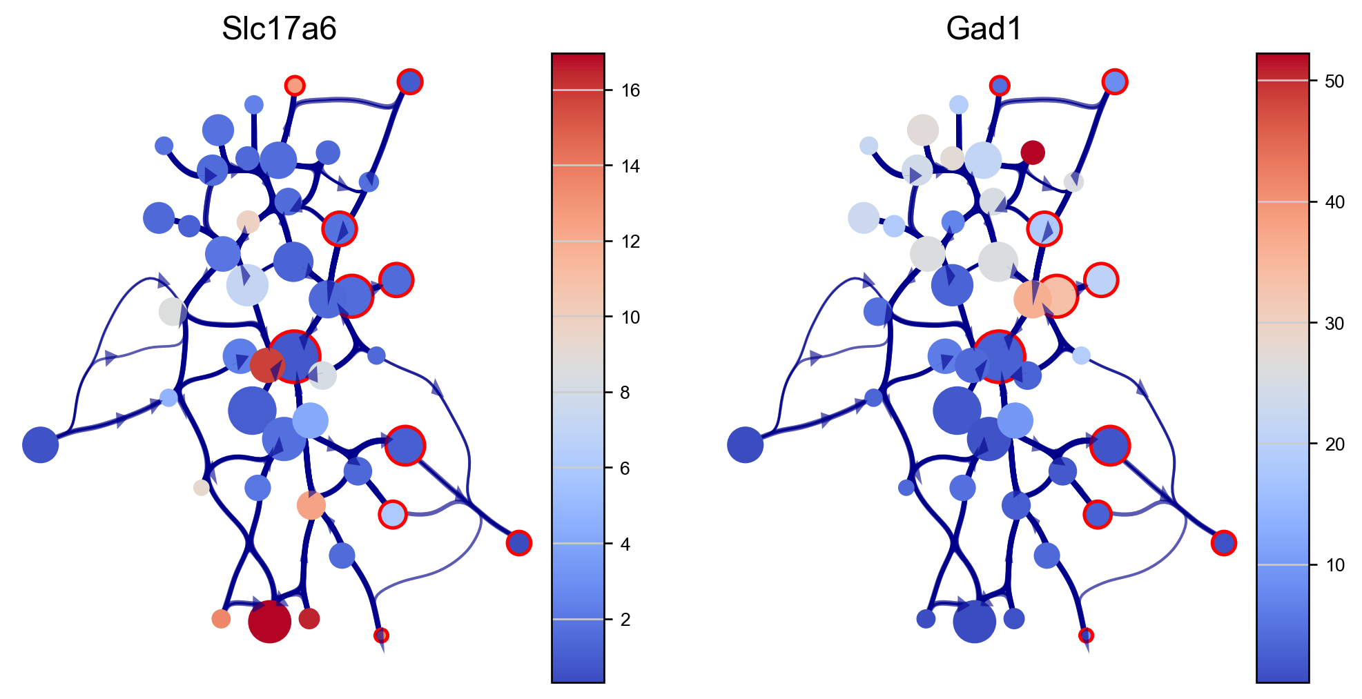
We can visualize genes expressions of our interest using the via graph (here we use excitatory and inibitory neuron markers SLC17A6 and GAD1). The via graph can be adjusted using parameters to tune the visualized connectivity between clusters. However, cell clustering are fixed once computed when executing via_object.run_VIA().
edgebundle_pruning-> high value increases number of visualized edges
initial_bandwidth-> higher value increases bundling of edges
decay-> higher value increases bundling of edges
genes=['Slc17a6', 'Gad1']
df_genes_sc = pd.DataFrame(adata[:, genes].X.todense(), columns=genes)
fig, axs=via.plot_viagraph(via_object=v0, df_genes=df_genes_sc, gene_list=genes, label_text=False,
tune_edges=True, edgebundle_pruning=0.7, decay=0.9, initial_bandwidth=0.05)
fig.set_size_inches(10,5)
plt.show()
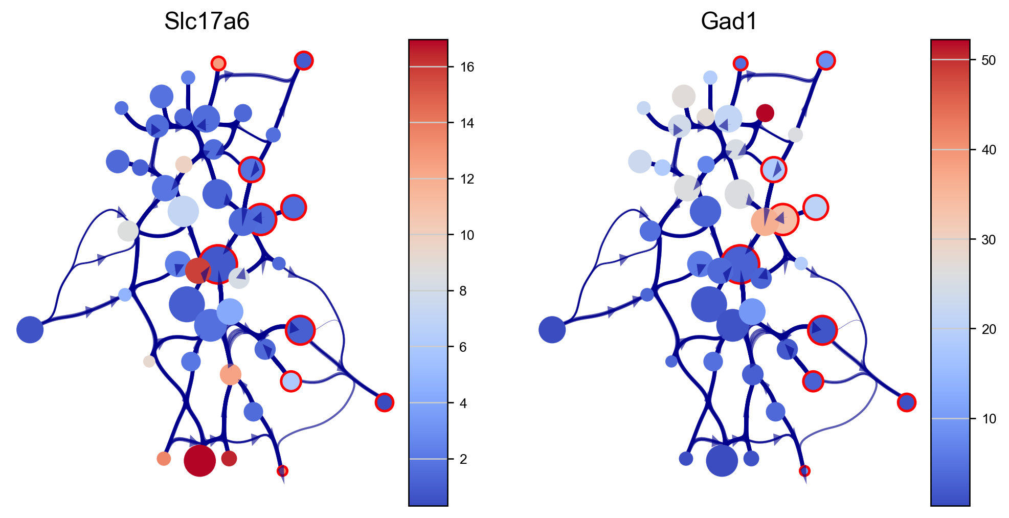
fig, axs=via.plot_viagraph(via_object=v0, df_genes=df_genes_sc, gene_list=genes, label_text=False,
tune_edges=True, edgebundle_pruning=0.9, decay=0.9, initial_bandwidth=0.05)
fig.set_size_inches(10,5)
plt.show()
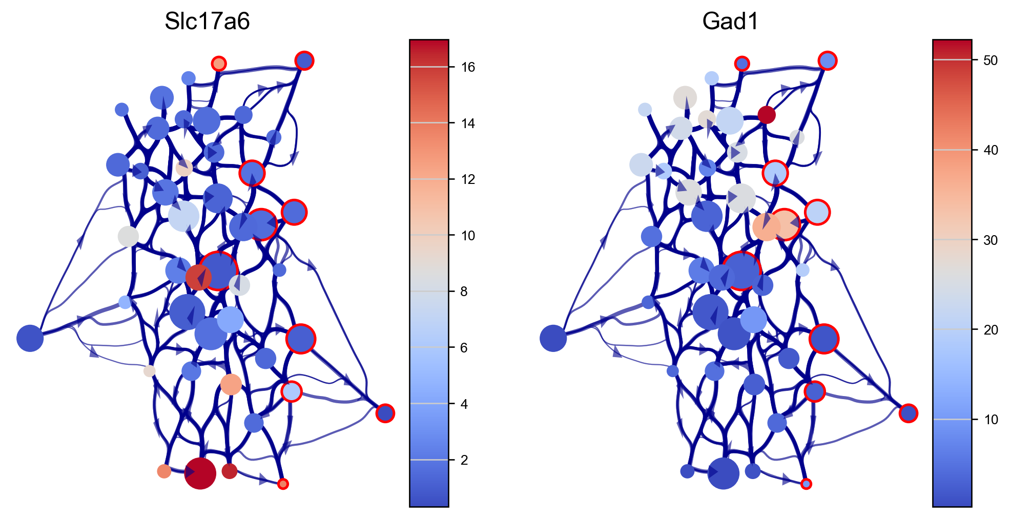
fig, axs=via.plot_viagraph(via_object=v0, df_genes=df_genes_sc, gene_list=genes, label_text=False,
tune_edges=True, edgebundle_pruning=0.7, decay=0.5, initial_bandwidth=0.05)
fig.set_size_inches(10,5)
plt.show()
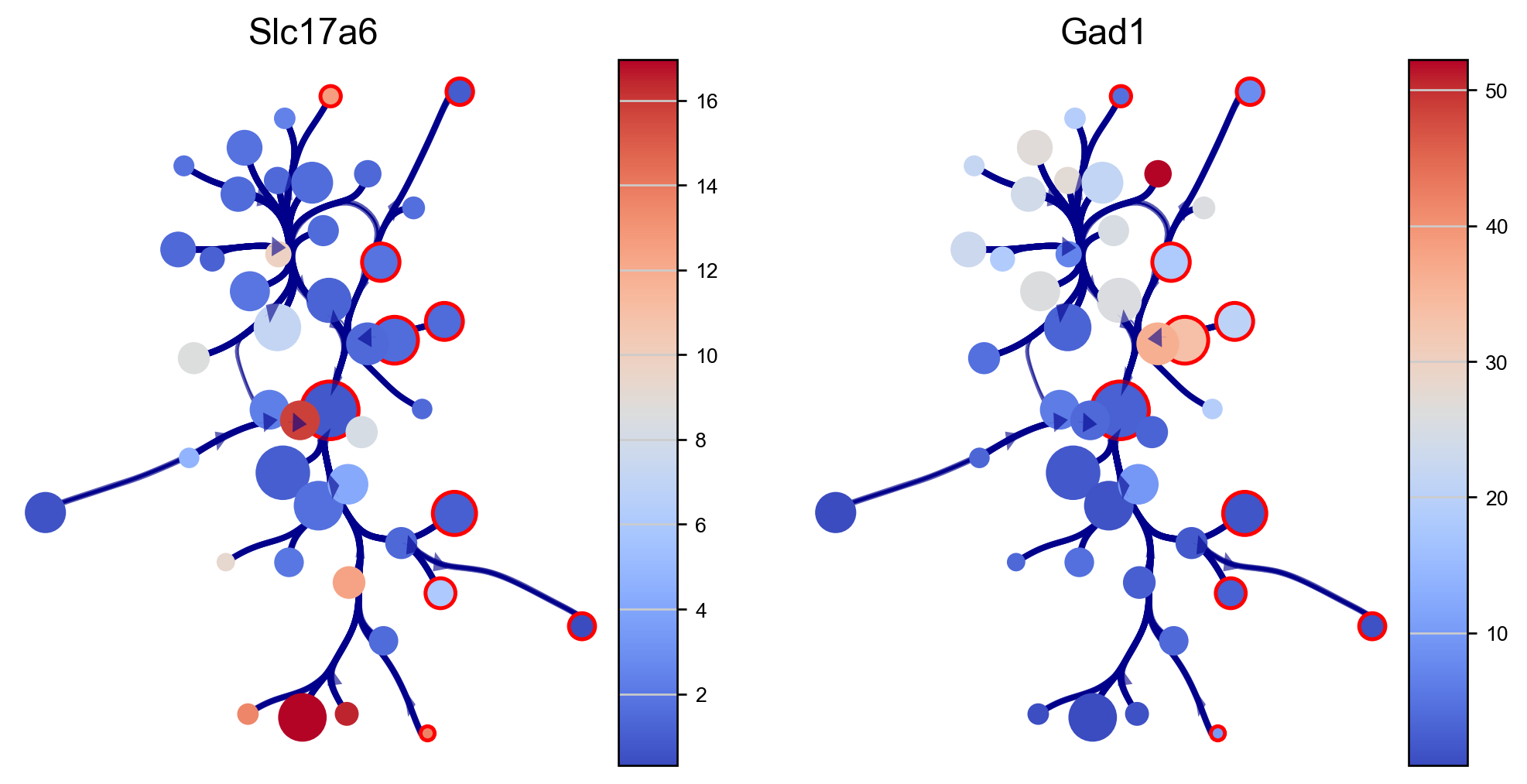
fig, axs=via.plot_viagraph(via_object=v0, df_genes=df_genes_sc, gene_list=genes, label_text=False,
tune_edges=True, edgebundle_pruning=0.7, decay=0.9, initial_bandwidth=0.1)
fig.set_size_inches(10,5)
plt.show()
2024-03-01 17:15:36.471237	Graph has 1 connected components before pruning
2024-03-01 17:15:36.471237	Graph has 1 connected components after pruning
2024-03-01 17:15:36.471237	Graph has 1 connected components after reconnecting
2024-03-01 17:15:36.486865	Make via clustergraph edgebundle
2024-03-01 17:15:38.154629	Hammer dims: Nodes shape: (44, 2) Edges shape: (1424, 3)
2024-03-01 17:15:43.368731	Graph has 1 connected components before pruning
2024-03-01 17:15:43.384329	Graph has 1 connected components after pruning
2024-03-01 17:15:43.384329	Graph has 1 connected components after reconnecting
2024-03-01 17:15:43.384329	Make via clustergraph edgebundle
2024-03-01 17:15:45.484062	Hammer dims: Nodes shape: (44, 2) Edges shape: (1706, 3)
2024-03-01 17:15:51.480837	Graph has 1 connected components before pruning
2024-03-01 17:15:51.480837	Graph has 1 connected components after pruning
2024-03-01 17:15:51.480837	Graph has 1 connected components after reconnecting
2024-03-01 17:15:51.496438	Make via clustergraph edgebundle
2024-03-01 17:15:52.898684	Hammer dims: Nodes shape: (44, 2) Edges shape: (1424, 3)
2024-03-01 17:15:58.248346	Graph has 1 connected components before pruning
2024-03-01 17:15:58.248346	Graph has 1 connected components after pruning
2024-03-01 17:15:58.248346	Graph has 1 connected components after reconnecting
2024-03-01 17:15:58.248346	Make via clustergraph edgebundle
2024-03-01 17:15:59.888822	Hammer dims: Nodes shape: (44, 2) Edges shape: (1424, 3)
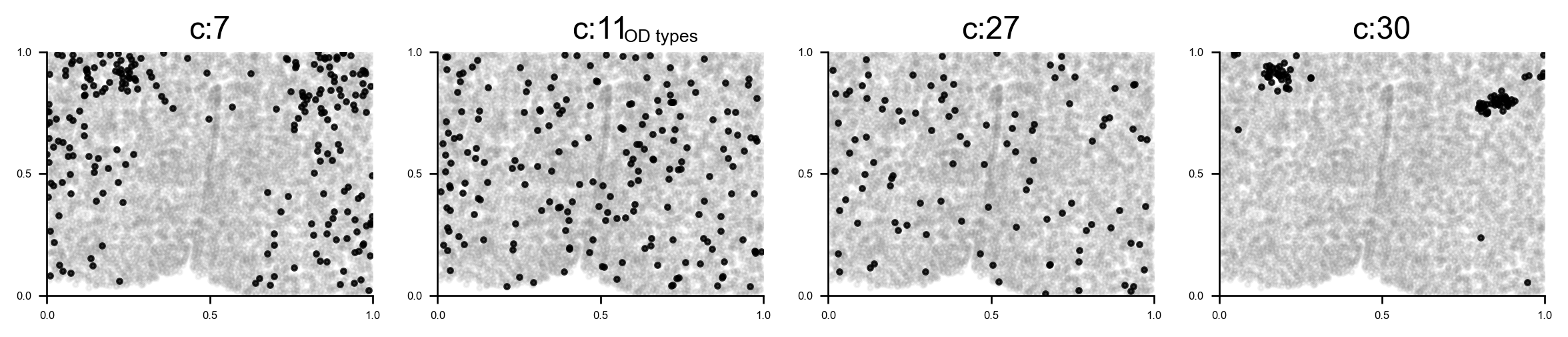
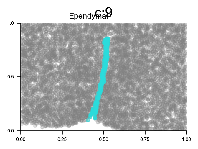
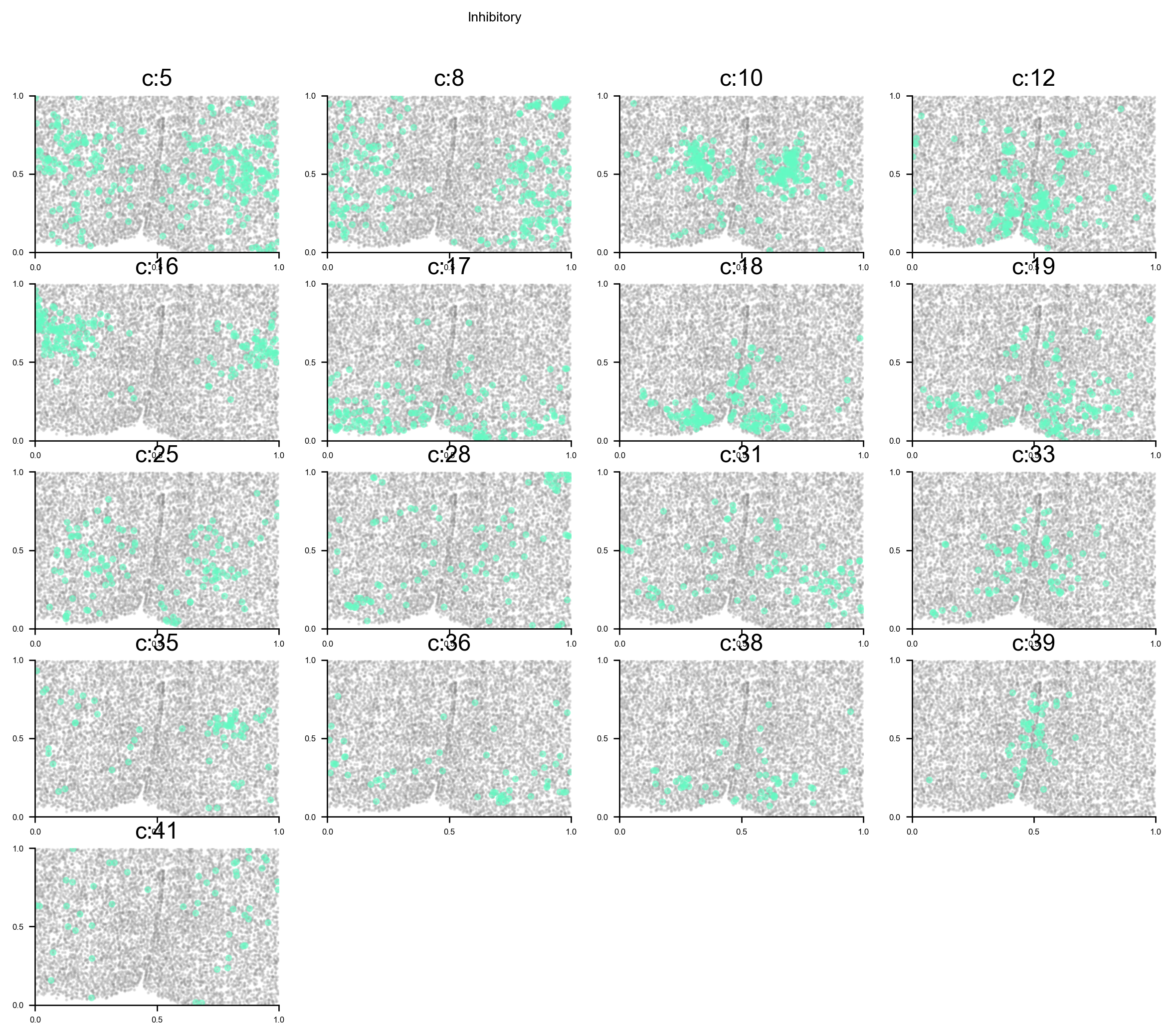
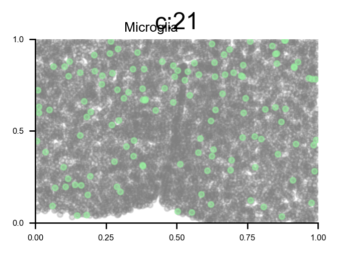
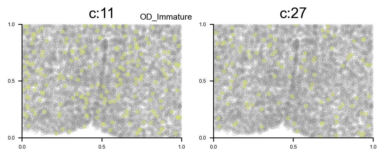
Reveal cell positions in tissue slice
We can highlight the cells positions in the tissue slice based on clusters.
# Plot selected clusters on the tissue slice
f, ax = via.plot_clusters_spatial(spatial_coords=coords, clusters = [7,11,27,30], color='black',
via_labels=v0.labels, title_sup='OD types', alpha = 0.8, s=5)
f.set_size_inches(12, 2)
plt.show()
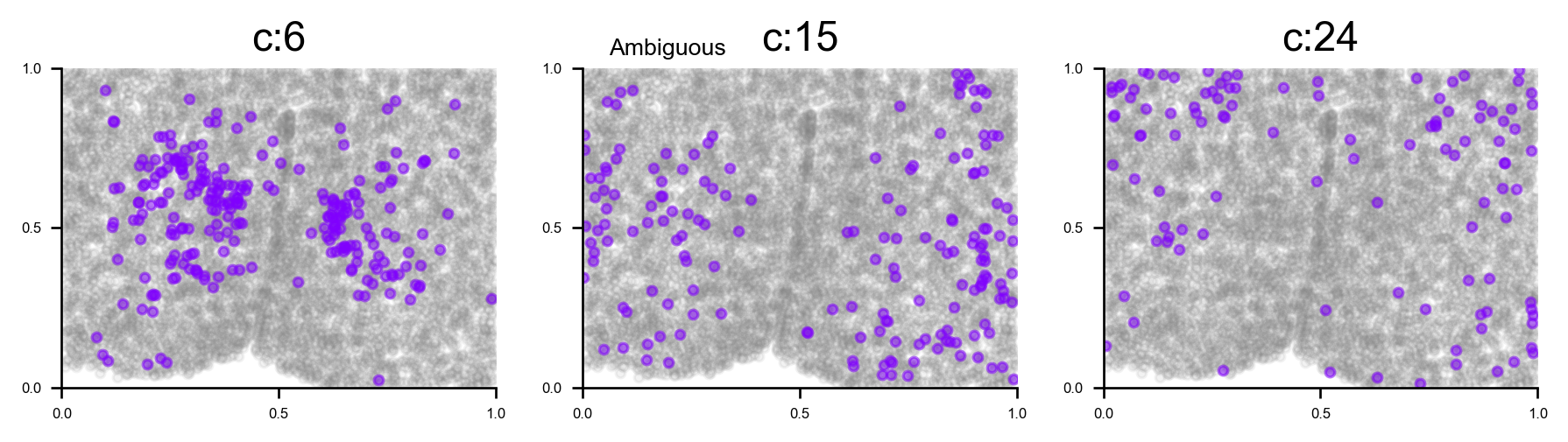
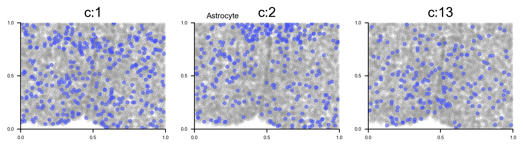
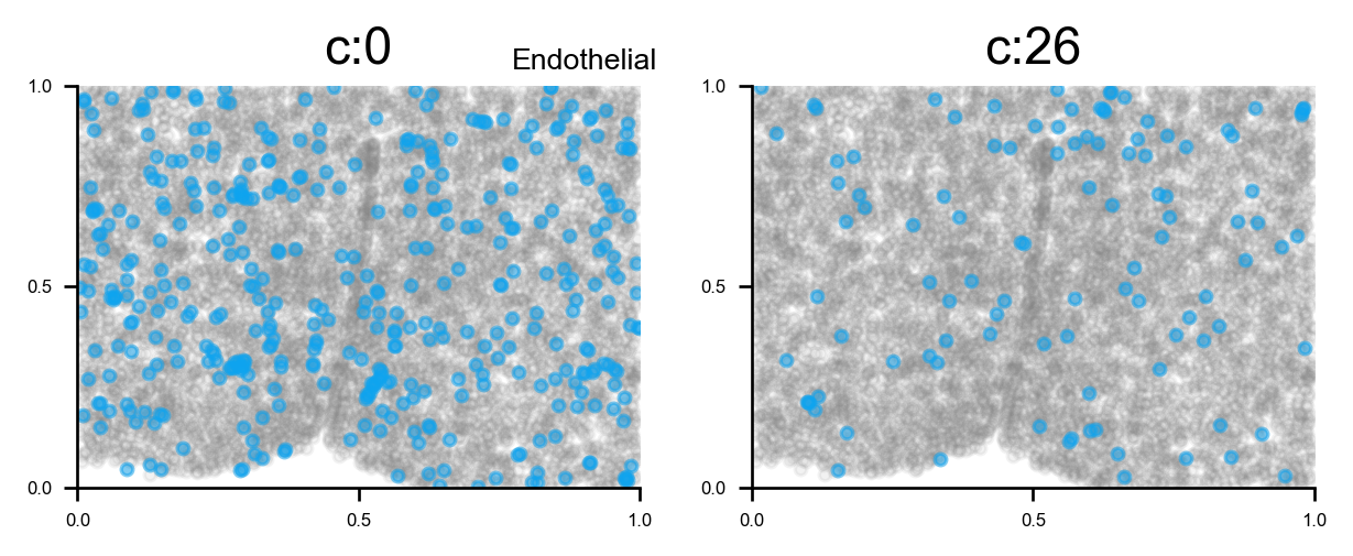
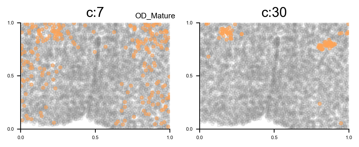
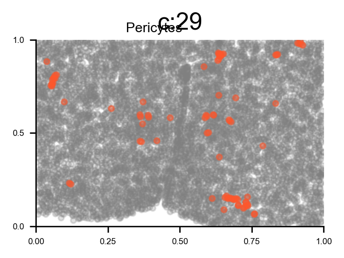
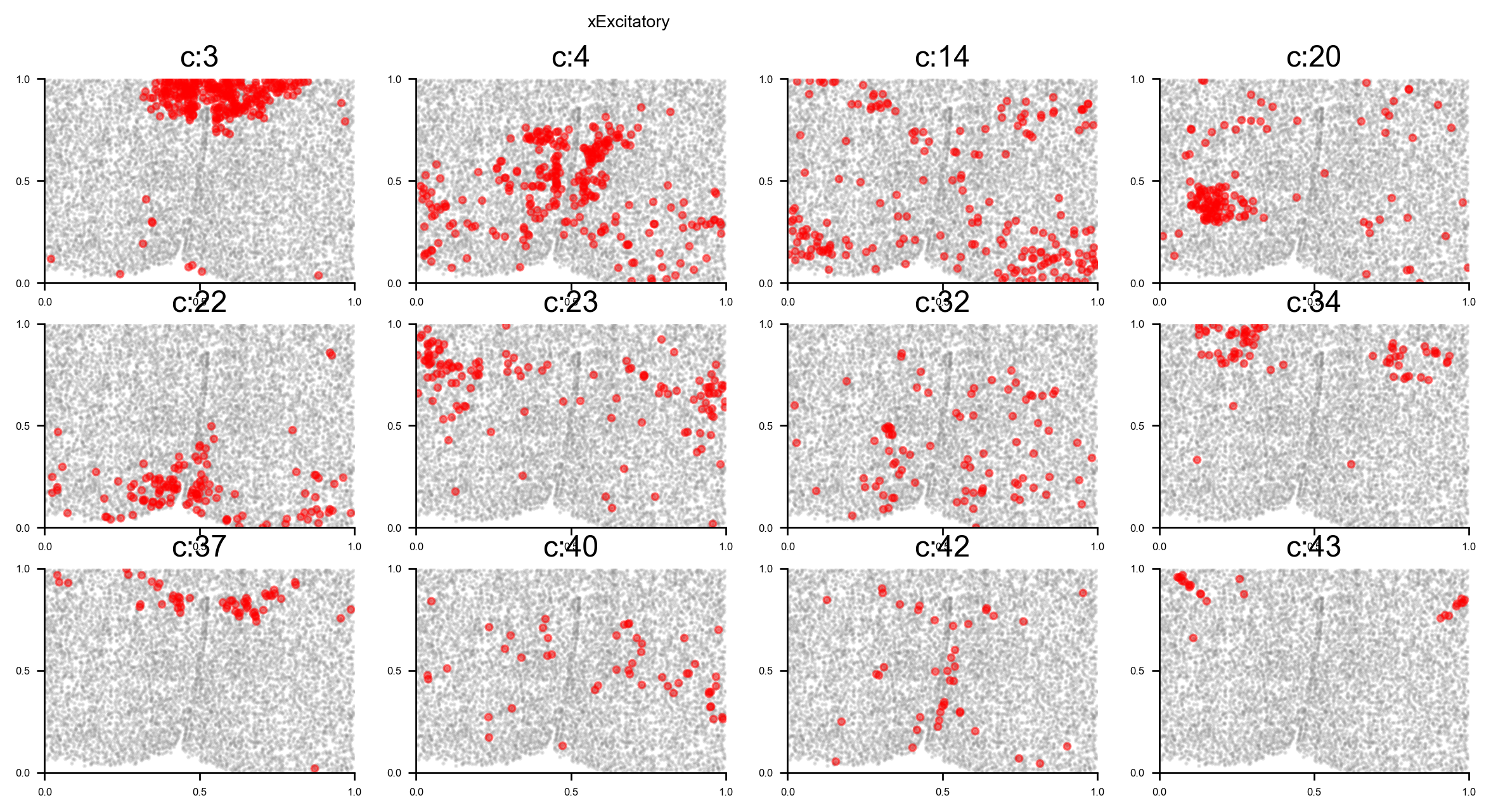
# plot all clusters on the tissue slices (one figure for each major cell type in True_label, and one subplot for each cluster)
f_ax_list = via.plot_all_spatial_clusters(spatial_coords= adata.obsm['spatial'], true_label=true_label,
via_labels=v0.labels, color_dict=color_dict, save_to=WORK_PATH,
verbose = False)
for f, ax in f_ax_list:
f.set_size_inches(3*np.clip(4,0,len(f.axes)), 2*(-(-len(f.axes)//4)))
plt.show()
No artists with labels found to put in legend. Note that artists whose label start with an underscore are ignored when legend() is called with no argument.
df_coords_majref  shape (6509, 2)
df_coords_majref  shape (6509, 2)
df_coords_majref  shape (6509, 2)
df_coords_majref  shape (6509, 2)
No artists with labels found to put in legend. Note that artists whose label start with an underscore are ignored when legend() is called with no argument.
dict cluster to majority pop: {0: 'Endothelial', 1: 'Astrocyte', 2: 'Astrocyte', 3: 'xExcitatory', 4: 'xExcitatory', 5: 'Inhibitory', 6: 'Ambiguous', 7: 'OD_Mature', 8: 'Inhibitory', 9: 'Ependymal', 10: 'Inhibitory', 11: 'OD_Immature', 12: 'Inhibitory', 13: 'Astrocyte', 14: 'xExcitatory', 15: 'Ambiguous', 16: 'Inhibitory', 17: 'Inhibitory', 18: 'Inhibitory', 19: 'Inhibitory', 20: 'xExcitatory', 21: 'Microglia', 22: 'xExcitatory', 23: 'xExcitatory', 24: 'Ambiguous', 25: 'Inhibitory', 26: 'Endothelial', 27: 'OD_Immature', 28: 'Inhibitory', 29: 'Pericytes', 30: 'OD_Mature', 31: 'Inhibitory', 32: 'xExcitatory', 33: 'Inhibitory', 34: 'xExcitatory', 35: 'Inhibitory', 36: 'Inhibitory', 37: 'xExcitatory', 38: 'Inhibitory', 39: 'Inhibitory', 40: 'xExcitatory', 41: 'Inhibitory', 42: 'xExcitatory', 43: 'xExcitatory'}
list of clusters for each majority {'Endothelial': [0, 26], 'Astrocyte': [1, 2, 13], 'xExcitatory': [3, 4, 14, 20, 22, 23, 32, 34, 37, 40, 42, 43], 'Inhibitory': [5, 8, 10, 12, 16, 17, 18, 19, 25, 28, 31, 33, 35, 36, 38, 39, 41], 'Ambiguous': [6, 15, 24], 'OD_Mature': [7, 30], 'Ependymal': [9], 'OD_Immature': [11, 27], 'Microglia': [21], 'Pericytes': [29]}
keys ['Ambiguous', 'Astrocyte', 'Endothelial', 'Ependymal', 'Inhibitory', 'Microglia', 'OD_Immature', 'OD_Mature', 'Pericytes', 'xExcitatory']
df_coords_majref  shape (6509, 2)
df_coords_majref  shape (6509, 2)
df_coords_majref  shape (6509, 2)
No artists with labels found to put in legend. Note that artists whose label start with an underscore are ignored when legend() is called with no argument.
df_coords_majref  shape (6509, 2)
df_coords_majref  shape (6509, 2)
df_coords_majref  shape (6509, 2)
No artists with labels found to put in legend. Note that artists whose label start with an underscore are ignored when legend() is called with no argument.
df_coords_majref  shape (6509, 2)
df_coords_majref  shape (6509, 2)
No artists with labels found to put in legend.  Note that artists whose label start with an underscore are ignored when legend() is called with no argument.
No artists with labels found to put in legend.  Note that artists whose label start with an underscore are ignored when legend() is called with no argument.
No artists with labels found to put in legend.  Note that artists whose label start with an underscore are ignored when legend() is called with no argument.
No artists with labels found to put in legend.  Note that artists whose label start with an underscore are ignored when legend() is called with no argument.
df_coords_majref  shape (6509, 2)
df_coords_majref  shape (6509, 2)
No artists with labels found to put in legend. Note that artists whose label start with an underscore are ignored when legend() is called with no argument.
df_coords_majref  shape (6509, 2)
df_coords_majref  shape (6509, 2)
No artists with labels found to put in legend.  Note that artists whose label start with an underscore are ignored when legend() is called with no argument.
No artists with labels found to put in legend.  Note that artists whose label start with an underscore are ignored when legend() is called with no argument.
do_rank_genes = True
adata.obs['parc_num'] = [i for i in v0.labels]
adata.obs['parc'] = [str(i) for i in v0.labels]
adata.strings_to_categoricals()
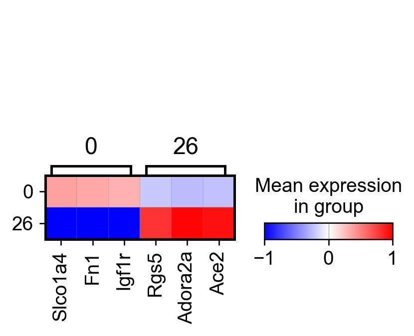
if do_rank_genes: # can also run this later, using via.labels clustering labels determined/saved after run_via()
print(adata.obsm['spatial'].shape)
adata.raw = adata
sc.pp.log1p(adata) # tl.rank_genes expects logarithmized data. If you want to see raw numbers then consider skipping this step
class_to_cluster_dict = via.make_dict_of_clusters_for_each_celltype(via_labels=v0.labels, true_label=true_label,
verbose=True)
for key in class_to_cluster_dict: # ['Astrocyte','Inhibitory','xExcitatory','Ambiguous',] or choose a subset of cell types
if len(class_to_cluster_dict[key]) == 1: continue
adata_ = adata[adata.obs['parc_num'].isin(class_to_cluster_dict[key])]
adata_.layers['scaled'] = sc.pp.scale(adata_, copy=True).X
print(adata_)
sc.tl.rank_genes_groups(adata_, groupby="parc", method='wilcoxon')#, use_raw=True)
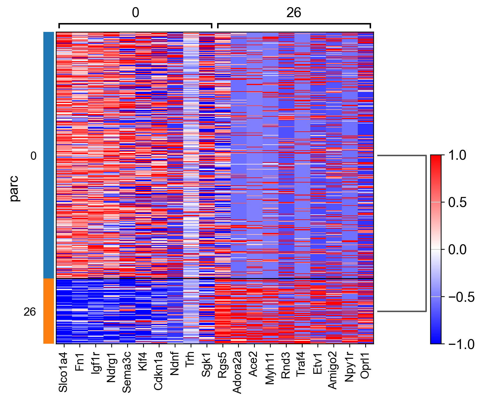
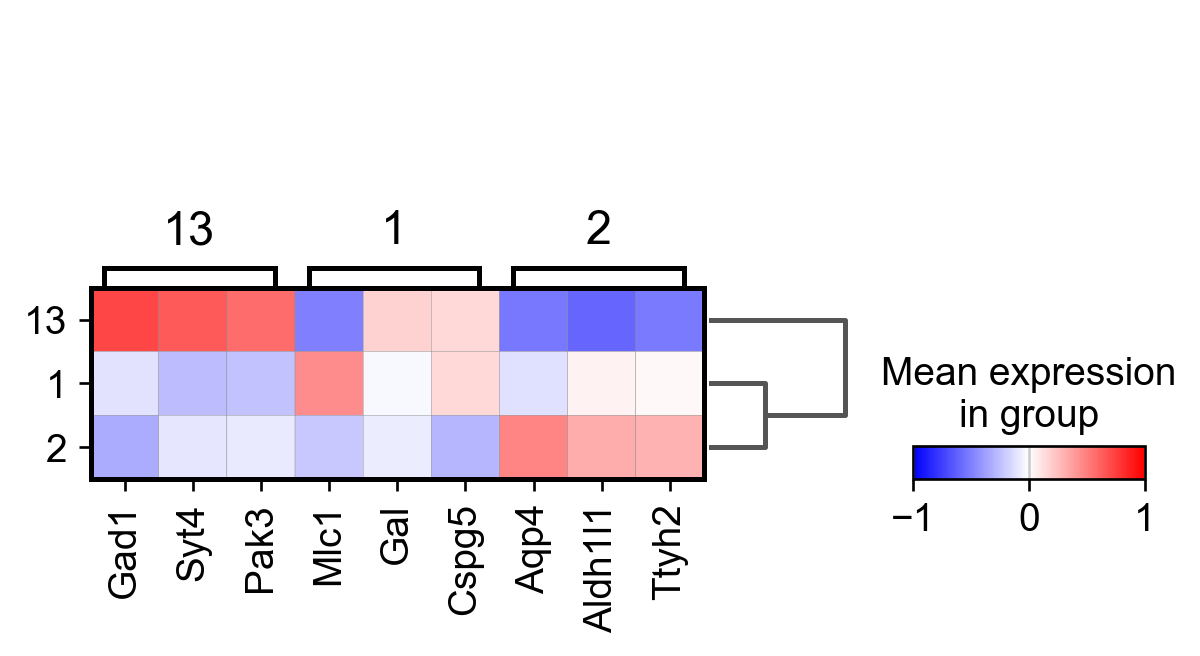
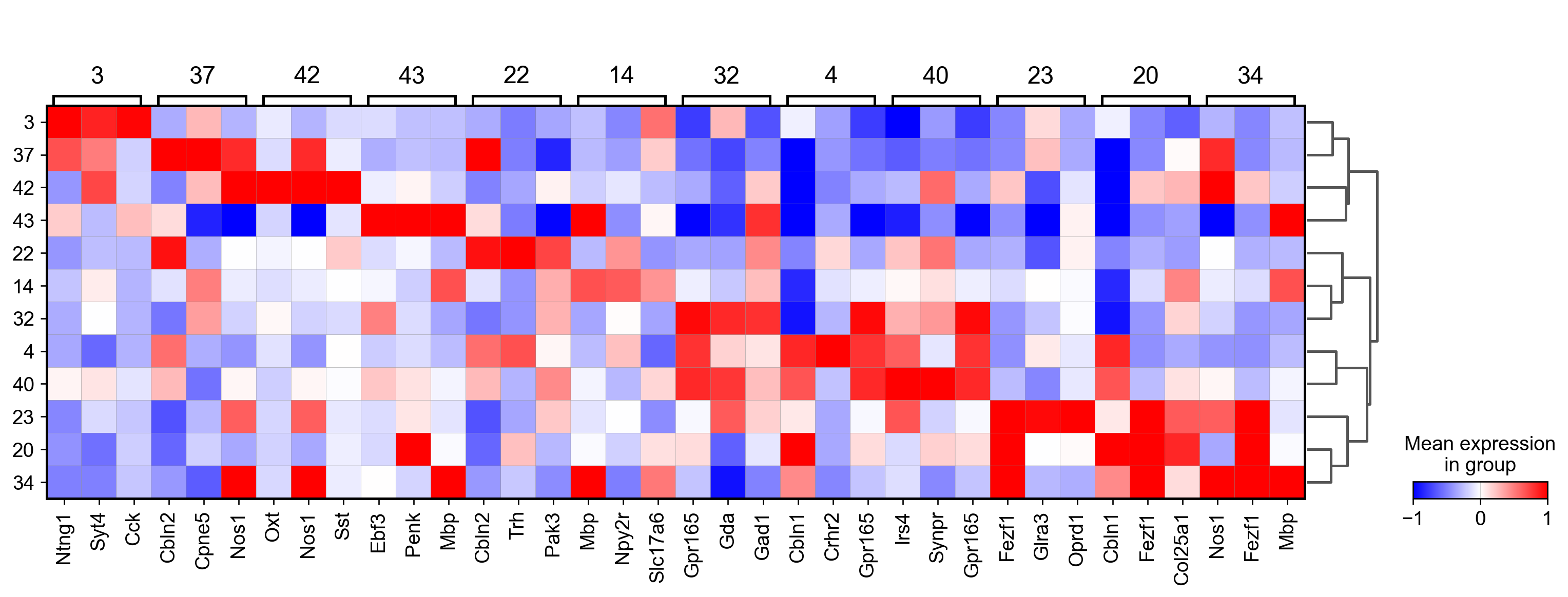
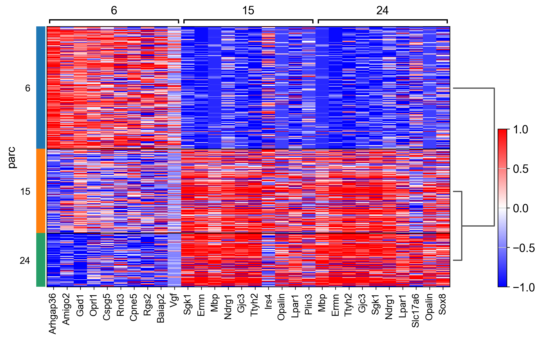
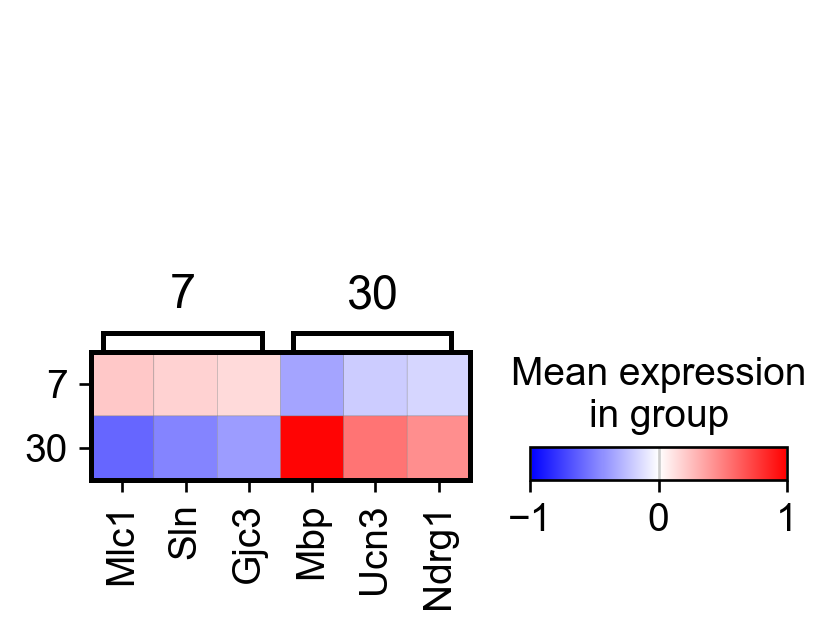
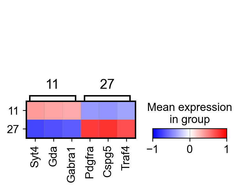
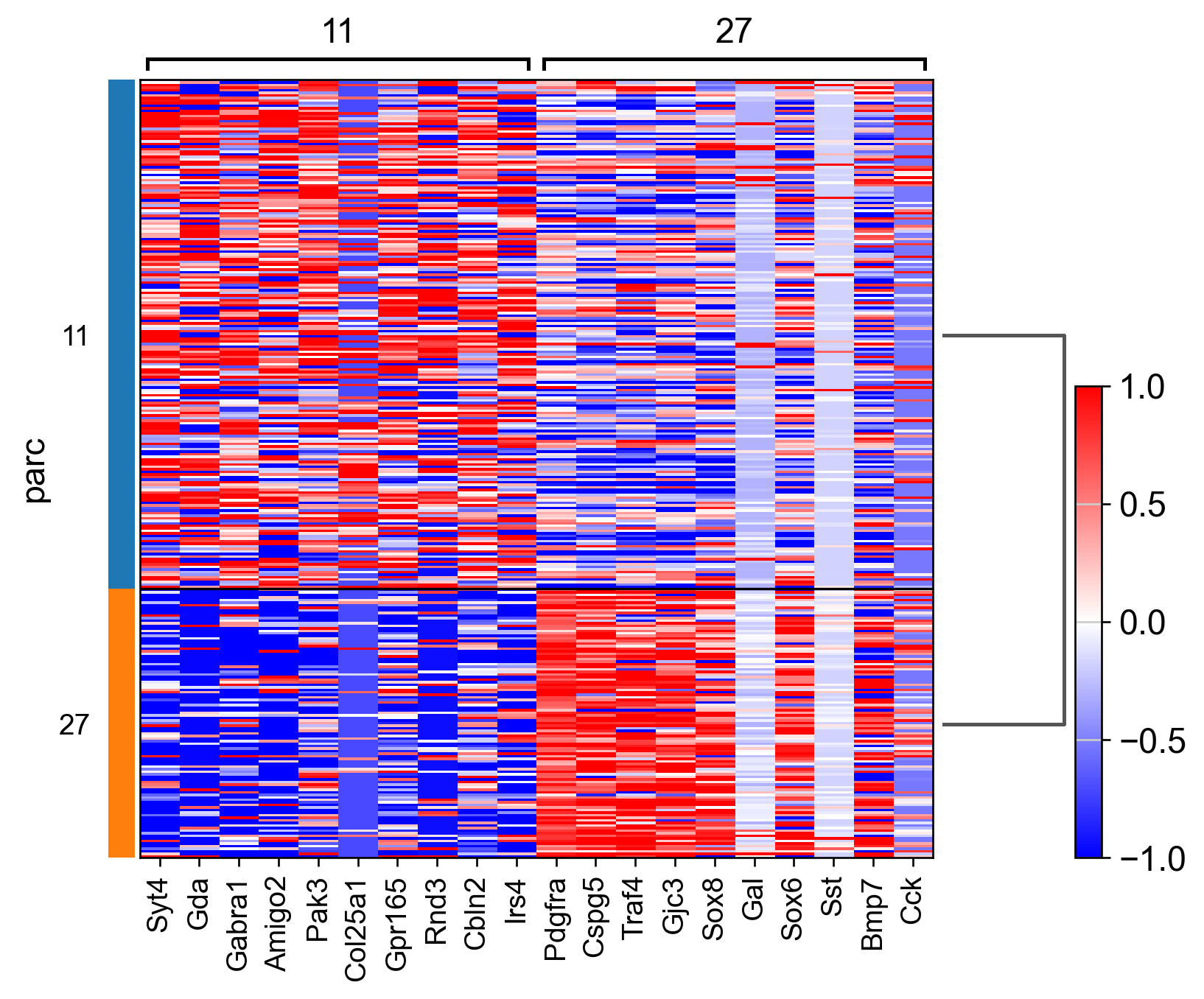
sc.pl.rank_genes_groups_matrixplot(adata_, n_genes=3, use_raw=False, vmin=-1, vmax=1, cmap='bwr', layer='scaled')
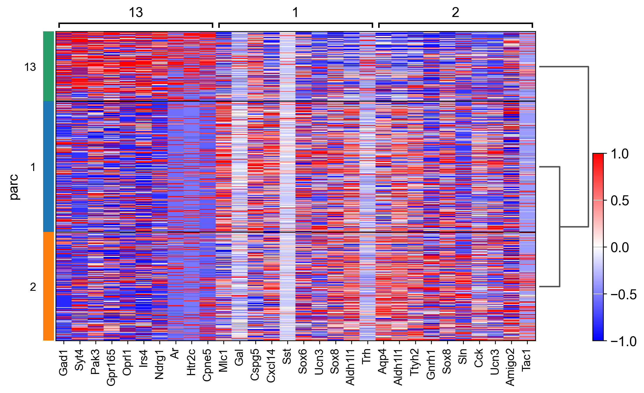
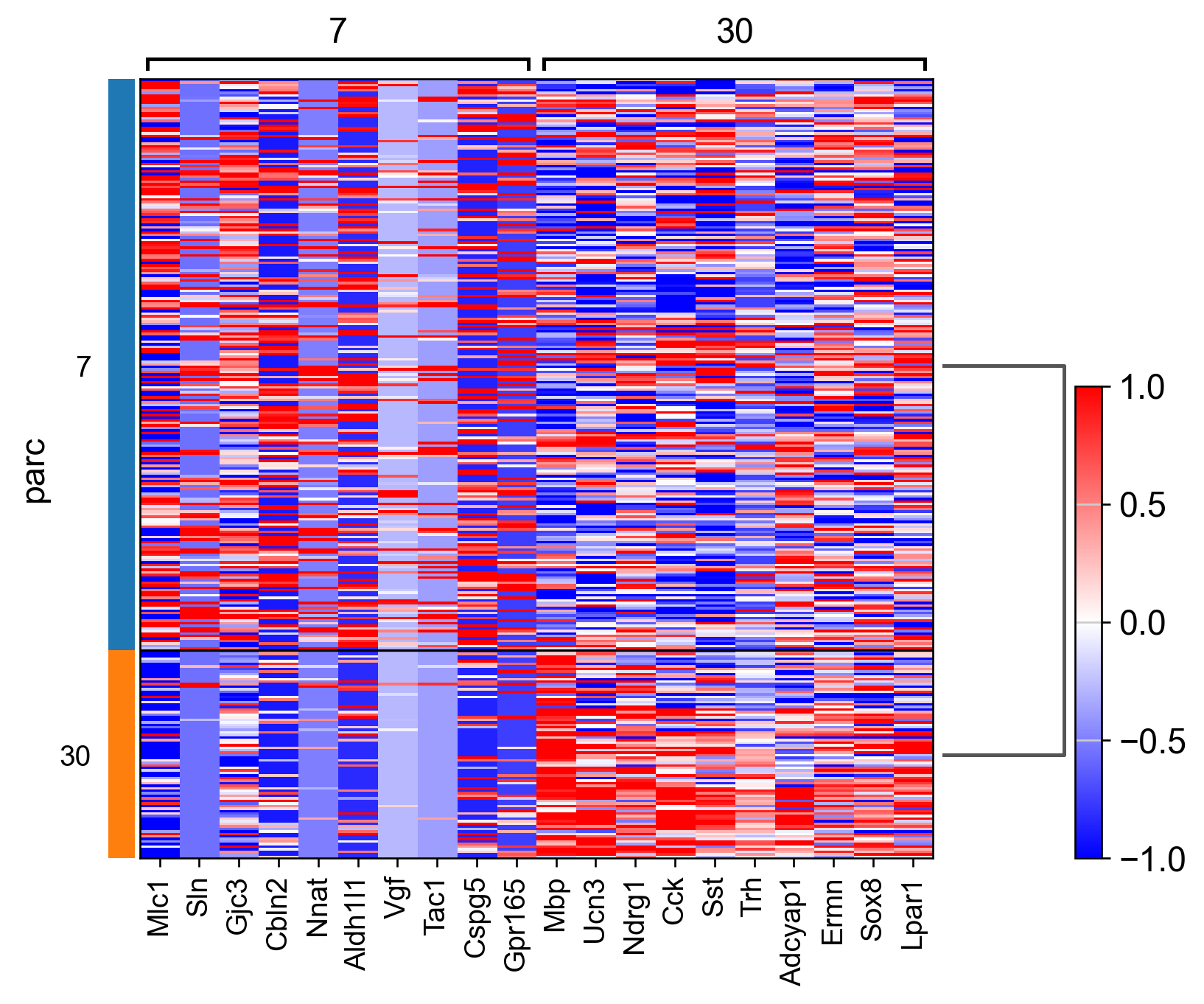
sc.pl.rank_genes_groups_heatmap(adata_, n_genes=10, show_gene_labels=True, cmap='bwr', vmin=-1,vmax=1, layer='scaled', use_raw=False)
(6509, 2)
dict cluster to majority pop: {0: 'Endothelial', 1: 'Astrocyte', 2: 'Astrocyte', 3: 'xExcitatory', 4: 'xExcitatory', 5: 'Inhibitory', 6: 'Ambiguous', 7: 'OD_Mature', 8: 'Inhibitory', 9: 'Ependymal', 10: 'Inhibitory', 11: 'OD_Immature', 12: 'Inhibitory', 13: 'Astrocyte', 14: 'xExcitatory', 15: 'Ambiguous', 16: 'Inhibitory', 17: 'Inhibitory', 18: 'Inhibitory', 19: 'Inhibitory', 20: 'xExcitatory', 21: 'Microglia', 22: 'xExcitatory', 23: 'xExcitatory', 24: 'Ambiguous', 25: 'Inhibitory', 26: 'Endothelial', 27: 'OD_Immature', 28: 'Inhibitory', 29: 'Pericytes', 30: 'OD_Mature', 31: 'Inhibitory', 32: 'xExcitatory', 33: 'Inhibitory', 34: 'xExcitatory', 35: 'Inhibitory', 36: 'Inhibitory', 37: 'xExcitatory', 38: 'Inhibitory', 39: 'Inhibitory', 40: 'xExcitatory', 41: 'Inhibitory', 42: 'xExcitatory', 43: 'xExcitatory'}
list of clusters for each majority {'Endothelial': [0, 26], 'Astrocyte': [1, 2, 13], 'xExcitatory': [3, 4, 14, 20, 22, 23, 32, 34, 37, 40, 42, 43], 'Inhibitory': [5, 8, 10, 12, 16, 17, 18, 19, 25, 28, 31, 33, 35, 36, 38, 39, 41], 'Ambiguous': [6, 15, 24], 'OD_Mature': [7, 30], 'Ependymal': [9], 'OD_Immature': [11, 27], 'Microglia': [21], 'Pericytes': [29]}
AnnData object with n_obs × n_vars = 507 × 161
    obs: 'Cell_ID', 'Animal_ID', 'Animal_sex', 'Behavior', 'Bregma', 'Centroid_X', 'Centroid_Y', 'Cell_class', 'Neuron_cluster_ID', 'batch', 'true_label', 'parc_num', 'parc'
    uns: 'Cell_class_colors', 'log1p'
    obsm: 'spatial', 'spatial3d', 'X_spatial_adjusted', 'spatial_pca'
    layers: 'scaled'
WARNING: Dendrogram not added. Dendrogram is added only when the number of categories to plot > 2
WARNING: dendrogram data not found (using key=dendrogram_parc). Running `sc.tl.dendrogram` with default parameters. For fine tuning it is recommended to run `sc.tl.dendrogram` independently.
WARNING: You’re trying to run this on 161 dimensions of `.X`, if you really want this, set `use_rep='X'`.
         Falling back to preprocessing with `sc.pp.pca` and default params.
AnnData object with n_obs × n_vars = 846 × 161
    obs: 'Cell_ID', 'Animal_ID', 'Animal_sex', 'Behavior', 'Bregma', 'Centroid_X', 'Centroid_Y', 'Cell_class', 'Neuron_cluster_ID', 'batch', 'true_label', 'parc_num', 'parc'
    uns: 'Cell_class_colors', 'log1p'
    obsm: 'spatial', 'spatial3d', 'X_spatial_adjusted', 'spatial_pca'
    layers: 'scaled'
WARNING: dendrogram data not found (using key=dendrogram_parc). Running `sc.tl.dendrogram` with default parameters. For fine tuning it is recommended to run `sc.tl.dendrogram` independently.
WARNING: You’re trying to run this on 161 dimensions of `.X`, if you really want this, set `use_rep='X'`.
         Falling back to preprocessing with `sc.pp.pca` and default params.
AnnData object with n_obs × n_vars = 1447 × 161
    obs: 'Cell_ID', 'Animal_ID', 'Animal_sex', 'Behavior', 'Bregma', 'Centroid_X', 'Centroid_Y', 'Cell_class', 'Neuron_cluster_ID', 'batch', 'true_label', 'parc_num', 'parc'
    uns: 'Cell_class_colors', 'log1p'
    obsm: 'spatial', 'spatial3d', 'X_spatial_adjusted', 'spatial_pca'
    layers: 'scaled'
WARNING: dendrogram data not found (using key=dendrogram_parc). Running `sc.tl.dendrogram` with default parameters. For fine tuning it is recommended to run `sc.tl.dendrogram` independently.
WARNING: You’re trying to run this on 161 dimensions of `.X`, if you really want this, set `use_rep='X'`.
         Falling back to preprocessing with `sc.pp.pca` and default params.
AnnData object with n_obs × n_vars = 2162 × 161
    obs: 'Cell_ID', 'Animal_ID', 'Animal_sex', 'Behavior', 'Bregma', 'Centroid_X', 'Centroid_Y', 'Cell_class', 'Neuron_cluster_ID', 'batch', 'true_label', 'parc_num', 'parc'
    uns: 'Cell_class_colors', 'log1p'
    obsm: 'spatial', 'spatial3d', 'X_spatial_adjusted', 'spatial_pca'
    layers: 'scaled'
WARNING: dendrogram data not found (using key=dendrogram_parc). Running `sc.tl.dendrogram` with default parameters. For fine tuning it is recommended to run `sc.tl.dendrogram` independently.
WARNING: You’re trying to run this on 161 dimensions of `.X`, if you really want this, set `use_rep='X'`.
         Falling back to preprocessing with `sc.pp.pca` and default params.
AnnData object with n_obs × n_vars = 523 × 161
    obs: 'Cell_ID', 'Animal_ID', 'Animal_sex', 'Behavior', 'Bregma', 'Centroid_X', 'Centroid_Y', 'Cell_class', 'Neuron_cluster_ID', 'batch', 'true_label', 'parc_num', 'parc'
    uns: 'Cell_class_colors', 'log1p'
    obsm: 'spatial', 'spatial3d', 'X_spatial_adjusted', 'spatial_pca'
    layers: 'scaled'
WARNING: dendrogram data not found (using key=dendrogram_parc). Running `sc.tl.dendrogram` with default parameters. For fine tuning it is recommended to run `sc.tl.dendrogram` independently.
WARNING: You’re trying to run this on 161 dimensions of `.X`, if you really want this, set `use_rep='X'`.
         Falling back to preprocessing with `sc.pp.pca` and default params.
AnnData object with n_obs × n_vars = 307 × 161
    obs: 'Cell_ID', 'Animal_ID', 'Animal_sex', 'Behavior', 'Bregma', 'Centroid_X', 'Centroid_Y', 'Cell_class', 'Neuron_cluster_ID', 'batch', 'true_label', 'parc_num', 'parc'
    uns: 'Cell_class_colors', 'log1p'
    obsm: 'spatial', 'spatial3d', 'X_spatial_adjusted', 'spatial_pca'
    layers: 'scaled'
WARNING: Dendrogram not added. Dendrogram is added only when the number of categories to plot > 2
WARNING: dendrogram data not found (using key=dendrogram_parc). Running `sc.tl.dendrogram` with default parameters. For fine tuning it is recommended to run `sc.tl.dendrogram` independently.
WARNING: You’re trying to run this on 161 dimensions of `.X`, if you really want this, set `use_rep='X'`.
         Falling back to preprocessing with `sc.pp.pca` and default params.
AnnData object with n_obs × n_vars = 304 × 161
    obs: 'Cell_ID', 'Animal_ID', 'Animal_sex', 'Behavior', 'Bregma', 'Centroid_X', 'Centroid_Y', 'Cell_class', 'Neuron_cluster_ID', 'batch', 'true_label', 'parc_num', 'parc'
    uns: 'Cell_class_colors', 'log1p'
    obsm: 'spatial', 'spatial3d', 'X_spatial_adjusted', 'spatial_pca'
    layers: 'scaled'
WARNING: Dendrogram not added. Dendrogram is added only when the number of categories to plot > 2
WARNING: dendrogram data not found (using key=dendrogram_parc). Running `sc.tl.dendrogram` with default parameters. For fine tuning it is recommended to run `sc.tl.dendrogram` independently.
WARNING: You’re trying to run this on 161 dimensions of `.X`, if you really want this, set `use_rep='X'`.
         Falling back to preprocessing with `sc.pp.pca` and default params.
Atlas View
Here we try and compute two different embeddings to construct the atlas views and compare those results.
VIA multidimensional scaling mds
VIA modified HNSW graph
# Extract cluster and cell type labels from via object to get major cell type population within each clusters.
df_mode = pd.DataFrame()
df_mode['cluster'] = v0.labels
df_mode['celltype'] = v0.true_label
majority_cluster_population_dict = df_mode.groupby(['cluster'])['celltype'].agg(
    lambda x: pd.Series.mode(x)[0])  # agg(pd.Series.mode would give all modes) #series
majority_cluster_population_dict = majority_cluster_population_dict.to_dict()
print(f'dict cluster to majority pop: {majority_cluster_population_dict}')
dict cluster to majority pop: {0: 'Endothelial', 1: 'Astrocyte', 2: 'Astrocyte', 3: 'xExcitatory', 4: 'xExcitatory', 5: 'Inhibitory', 6: 'Ambiguous', 7: 'OD_Mature', 8: 'Inhibitory', 9: 'Ependymal', 10: 'Inhibitory', 11: 'OD_Immature', 12: 'Inhibitory', 13: 'Astrocyte', 14: 'xExcitatory', 15: 'Ambiguous', 16: 'Inhibitory', 17: 'Inhibitory', 18: 'Inhibitory', 19: 'Inhibitory', 20: 'xExcitatory', 21: 'Microglia', 22: 'xExcitatory', 23: 'xExcitatory', 24: 'Ambiguous', 25: 'Inhibitory', 26: 'Endothelial', 27: 'OD_Immature', 28: 'Inhibitory', 29: 'Pericytes', 30: 'OD_Mature', 31: 'Inhibitory', 32: 'xExcitatory', 33: 'Inhibitory', 34: 'xExcitatory', 35: 'Inhibitory', 36: 'Inhibitory', 37: 'xExcitatory', 38: 'Inhibitory', 39: 'Inhibitory', 40: 'xExcitatory', 41: 'Inhibitory', 42: 'xExcitatory', 43: 'xExcitatory'}
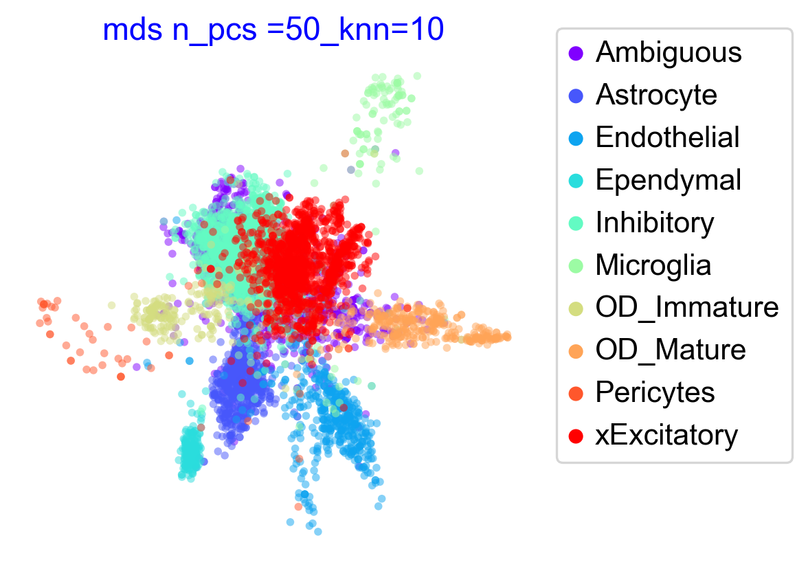
VIA mds embedding
Fast comupatation methods of a embedding thus compatible with highly scaled datasets and suitable for testing out numerous parameters.
mds_title = 'mds n_pcs ='+str(n_pcs) +'_knn='+str(knn)
emb_mds = via.via_mds(via_object=v0, n_milestones=5000)

f1, ax1 = via.plot_scatter(embedding=emb_mds, labels=true_label, title=mds_title, alpha=0.5,s=12,show_legend=True,color_dict=color_dict, text_labels=False)
ax1.get_legend().set_bbox_to_anchor((1.05, 1.05))
plt.show()
2024-03-01 17:16:32.752399	Commencing Via-MDS
minrowznormed -7874.4873
2024-03-01 17:16:35.362182	Start computing with diffusion power:1
2024-03-01 17:16:35.811552	Starting MDS on milestone
2024-03-01 17:16:56.161209	End computing mds with diffusion power:1
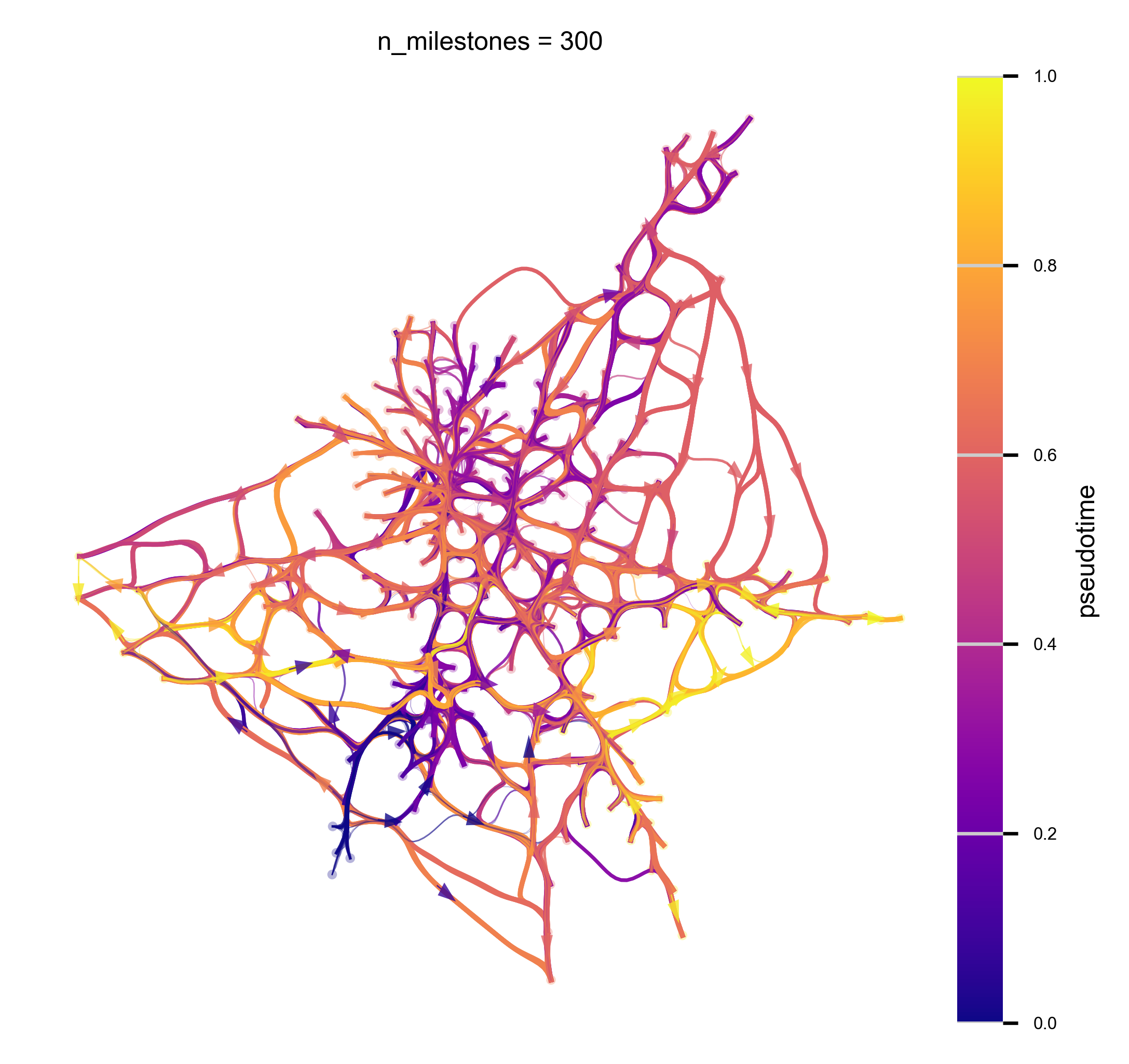
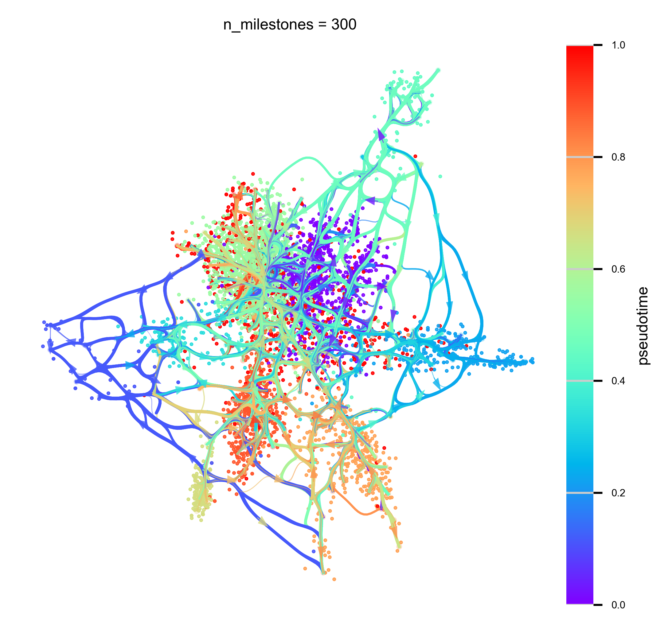
n_milestones = 300
i_bw = 0.03
decay=0.6
global_visual_pruning = 0.6
v0.embedding =emb_mds#emb
sc_scatter_alpha=0.4
sc_scatter_size=0.2
headwidth_bundle = 0.01
linewidth_bundle = 1
hammerbundle_dict = via.make_edgebundle_milestone(via_object=v0, n_milestones=n_milestones, decay=decay,
                                                  initial_bandwidth=i_bw, global_visual_pruning=global_visual_pruning)
v0.hammerbundle_milestone_dict = hammerbundle_dict  # make the hmbd in one shot to be used for all plots

f,ax = via.plot_atlas_view(via_object=v0, add_sc_embedding=True, sc_labels_expression=true_label, sc_labels=true_label,
                           sc_scatter_size=sc_scatter_size, sc_scatter_alpha=sc_scatter_alpha,
                           cmap='rainbow', linewidth_bundle=linewidth_bundle,
                           headwidth_bundle=headwidth_bundle)
plt.show()

f,ax = via.plot_atlas_view(via_object=v0, add_sc_embedding=True, sc_labels=true_label,
                           sc_scatter_size=sc_scatter_size, sc_scatter_alpha=sc_scatter_alpha,
                           cmap='plasma', linewidth_bundle=linewidth_bundle,
                           headwidth_bundle=headwidth_bundle)
plt.show()
2024-03-01 17:16:56.455572	Start finding milestones
2024-03-01 17:16:58.151925	End milestones with 300
2024-03-01 17:16:58.151925	Recompute weights
2024-03-01 17:16:58.198796	pruning milestone graph based on recomputed weights
2024-03-01 17:16:58.198796	Graph has 1 connected components before pruning
2024-03-01 17:16:58.198796	Graph has 1 connected components after pruning
2024-03-01 17:16:58.198796	Graph has 1 connected components after reconnecting
2024-03-01 17:16:58.214419	regenerate igraph on pruned edges
2024-03-01 17:16:58.261290	Setting numeric label as single cell pseudotime for coloring edges
2024-03-01 17:16:58.323785	Making smooth edges
inside add sc embedding second if
inside add sc embedding second if